Adaptive Asset Allocation – Resolve

Today’s post looks at a paper from ReSolve Asset Management on Adaptive Asset Allocation.
Contents
Adaptive Asset Allocation
We’ve met ReSolve several times before, but this is the first time that we’ve looked at Adaptive Asset Allocation (AAA).

![]()
The guys at ReSolve are no strangers to the topic – they wrote a book about it, which was published in 2016.
- I might look at that book in the future, but for today we have a 16-page white paper to examine.
Modern Portfolio Theory
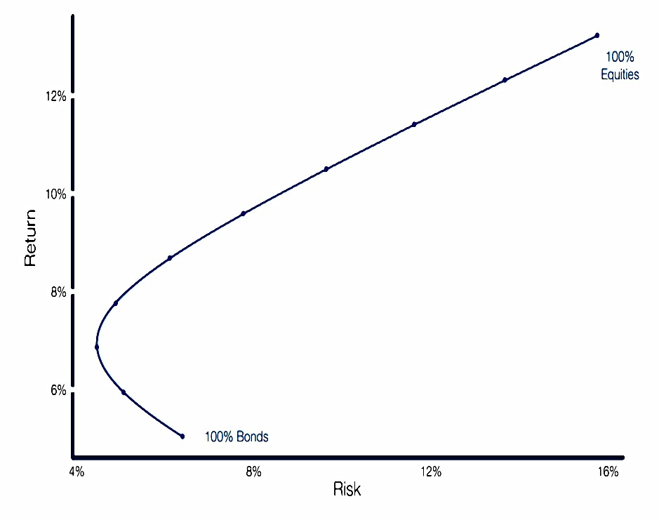
The paper begins with a look at Modern Portfolio Theory (MPT) (( I think it’s a shame that we’re stuck with that name since the theory is now seventy years old )) and the efficient frontier for a stock/bond portfolio.
- MPT is all about efficiency and getting the most out of the benefits of diversification.
It works out the allocation which provides the most return for a given level of risk (volatility).
- The continuum of all such portfolios is the efficient frontier.
Unfortunately, MPT is very sensitive to user and data error – “garbage in, garbage out” (GIGO).
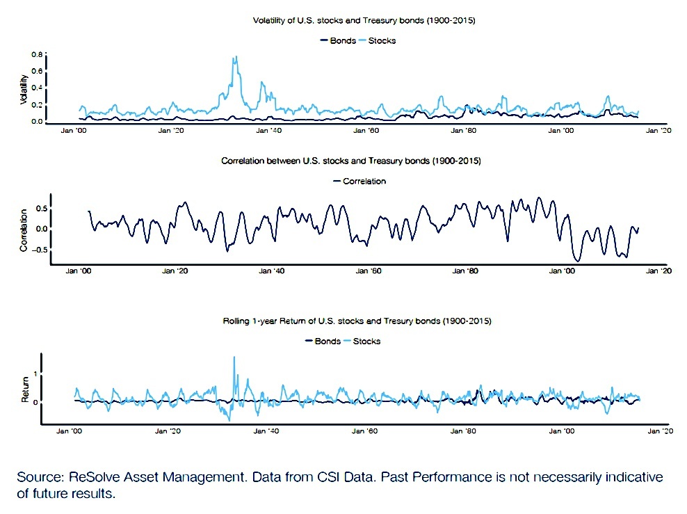
Some of this is down to volatility.
Traditional approaches to asset allocation assume that assets will always act in accordance with their long-term average behavior – steady returns with stable risk, and consistent relationships with one another. A simple observation of asset class behavior through history quickly dispels this illusion.
Asset classes
AAA is designed to add information from the recent past in order to improve allocations.
To show how the process works, ReSolve looked at 10 global asset classes, using data back to 1995:
- U.S. stocks
- European stocks
- Japanese stocks
- Emerging market stocks
- U.S. REITs
- International REITs
- U.S. 7-10 year Treasuries
- U.S. 20+ year Treasuries
- Commodities
- Gold
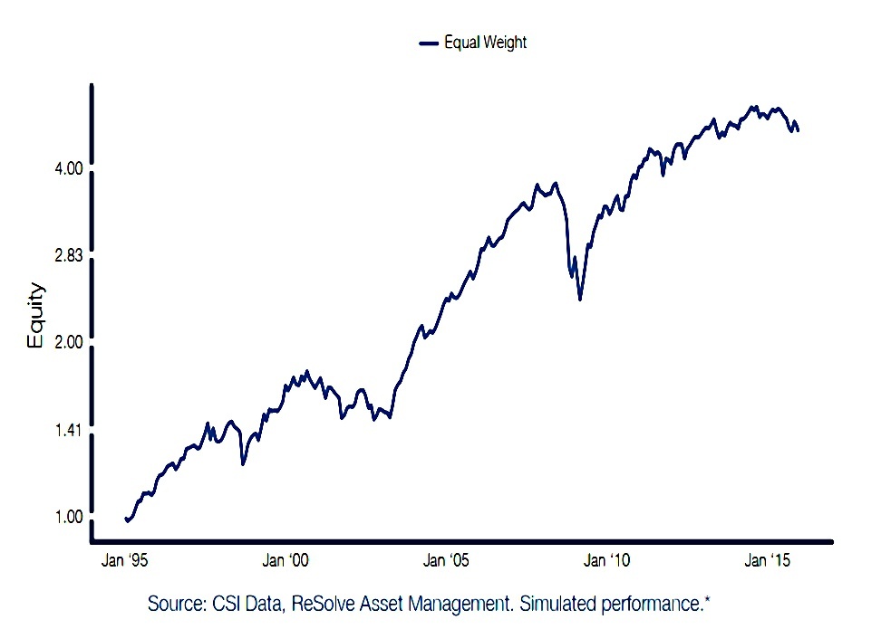
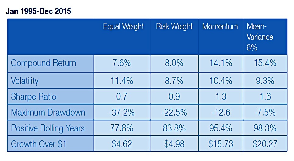
The baseline is an equal-weighted portfolio, which did fine – 7.6% pa returns, 11.4% vol, Sharpe of 0.7.
- The Max Drawdown (in 2008-09) is not so good, at -37%.
Vol weighting
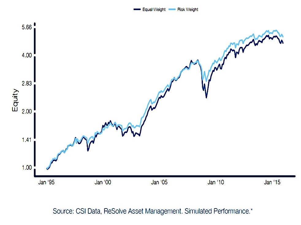
The first improvement is monthly volatility rebalancing, to give bonds more chance to impact returns.
- The lookback period for volatility was 60 days.
In the equally weighted case, the portfolio’s risk is overwhelmingly determined by higher volatility assets in the portfolio, like stocks, REITs and commodities.
Returns increase to 8.0% pa, volatility reduced to 8.7% and the Sharpe went up to 0.9.
- Max drawdown went down to -22.5%.
Momentum
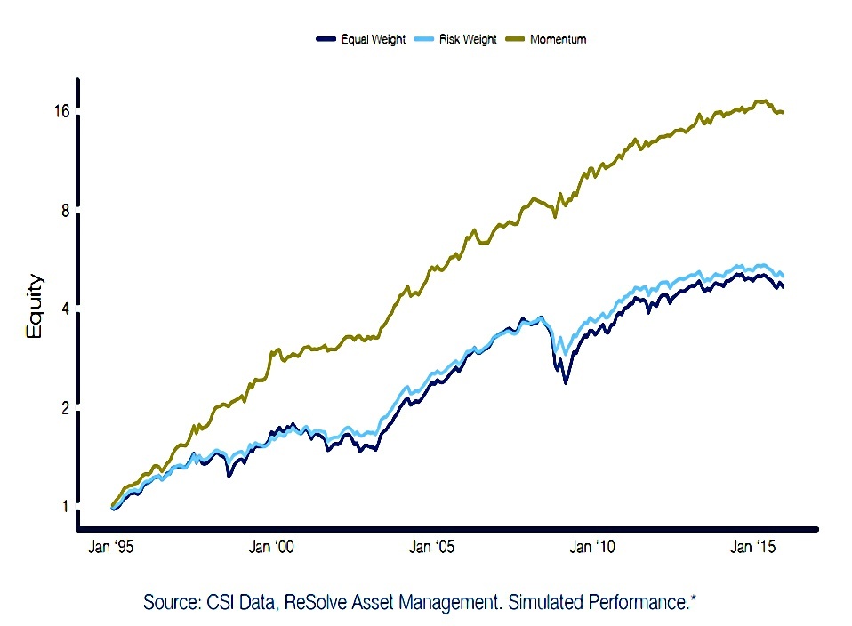
ReSolve see volatility rebalancing as portfolio defence.
- Their first dose of offence is momentum, which they use to generate estimates of expected future returns.
A six-month lookback was used and the top five assets from the list of ten were chosen.
- Note that volatility rebalancing from the previous step was maintained – these steps are additive.
There’s a big improvement here – returns are 14.1% pa, Sharpe is up to 1.3 and max drawdown falls to -12.6%.
Correlations
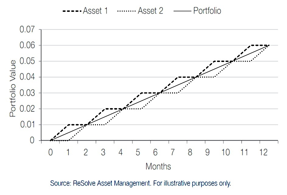
So far, we’ve ignored correlations.
Two risky assets with equal volatility and perfect negative correlation can be combined to form a portfolio with zero volatility and a positive return.
Of course, that’s an extreme example.
By using multiple momentum look-back periods, and MPT rules for assembling assets with low correlations, ReSolve find the portfolios with the highest momentum at their target level of volatility:
Portfolios with strong momentum, and which account for asset class risks and correlations, are reformed each month from assets in the top half by momentum across multiple historical periods, such that they produce the maximum momentum achievable with 8% portfolio volatility.
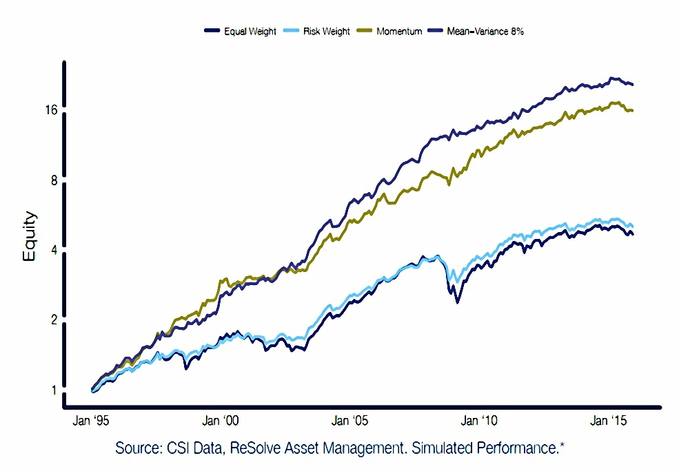
This leads to further small improvements across the board:
- returns are up to 15.4% pa, volatility is down to 9.3%, Sharpe is up to 1.6 and max drawdown is just -7.5% (on a month-end basis).
We also have positive returns from 98.3% of rolling 12-month periods.
Capital market line
While this portfolio may meet the needs of a large portion of investors, many investors have a preference for higher returns and can tolerate more risk. Fortunately, it’s easy to meet the objectives of almost any investor by employing the Capital Market Line (CML).
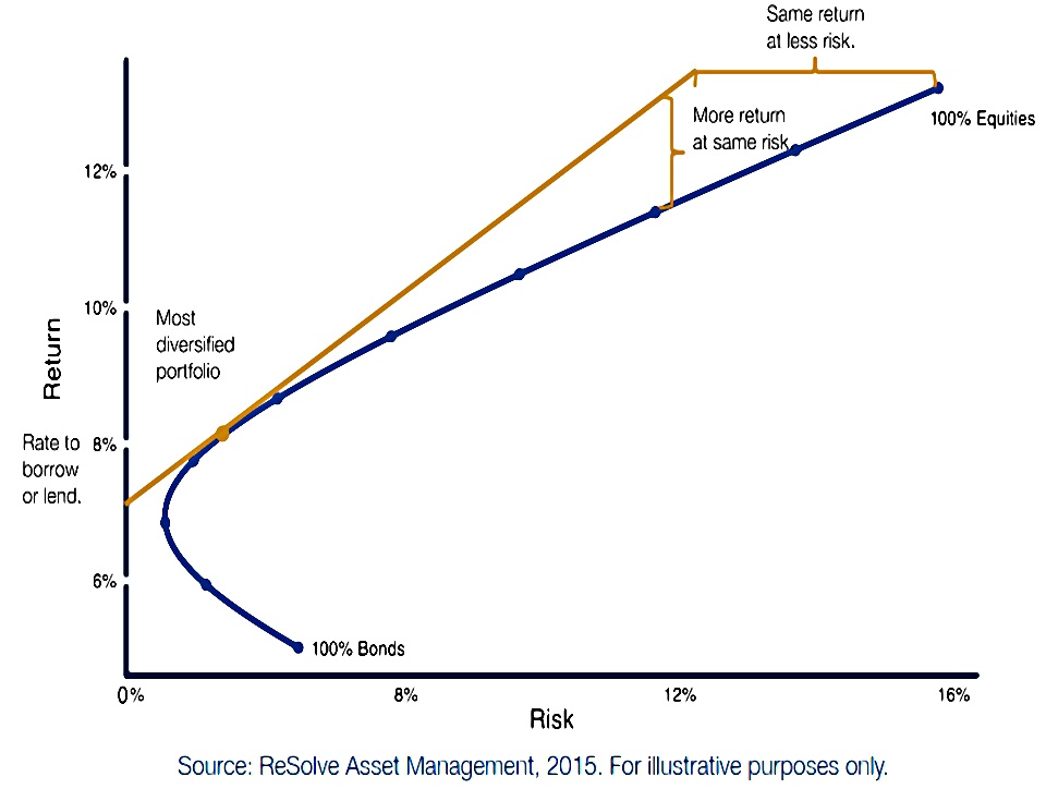
This basically means that if you can borrow at a rate lower than the return on the portfolio (which, given that we now have a portfolio with 15.4% pa returns, most people should be able to) you can scale up exposure to meet any higher return target.
- A similar approach can be used to achieve a given level of return with lower risk (by choosing a more stable base portfolio).
12% Vol
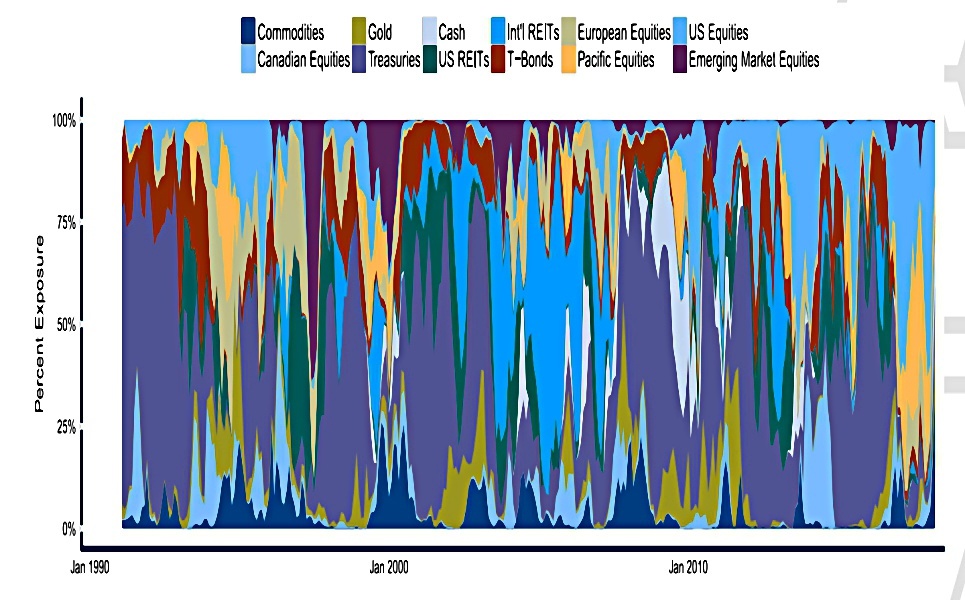
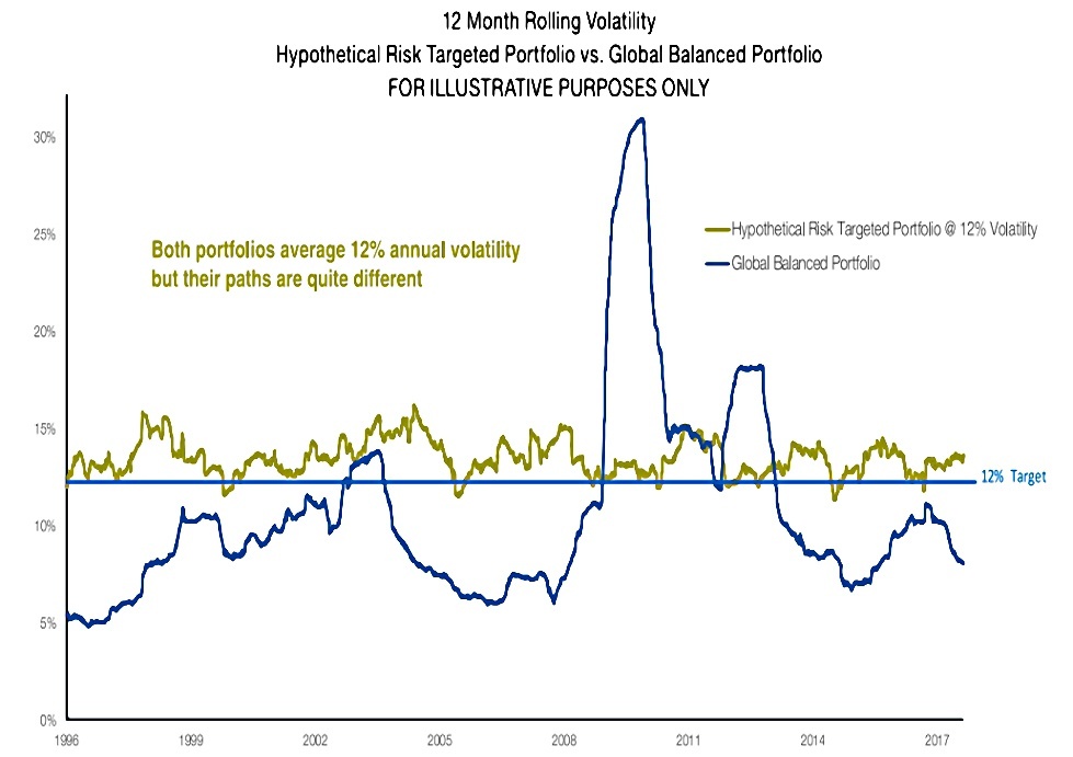
A companion flyer to ReSolve’s AAA offering looks at a similar portfolio targeting 12% volatility and includes a couple of interesting charts.
- The chart above shows how the asset allocations evolve during a thirty-year period
- The chart below demonstrates how the risk-targeted portfolio sticks closely to its volatility target whilst the global balanced portfolio swings around wildly.
That’s it for today – it’s been a refreshingly accessible paper with some interesting results.
- The next step for me is to give some thought to how best to implement these ideas as a private investor.
We’ll also look at some other papers on AAA, from a variety of sources.
- Until next time.
Mike Rawson
Mike is the owner of 7 Circles, and a private investor living in London. He has been managing his own money for 40 years, with some success.