Systematic Trading 6 – Practice
Today’s post is our sixth visit to Robert Carver’s book Systematic Trading.
Contents
Semi-automatic trader

In the final section of his book, Rob gives examples of how the three different kinds of investor should use his framework.
First up is the semi-automatic trader, who makes his own calls on the market.
- They can focus on the buy/sell decision, and let the system take care of stop losses, risk targeting and position sizing.
Rob assumes that this trader is trading spread bets on equity indices and FX with £100K of capital.
- Bet sizes will usually be between £1 and £10 per point.
- Costs should be less than 0.01 Sharpe Ratio units and any position should be a minimum of four instrument blocks.
Stop losses
Rob uses a stop-loss set at a multiple of the daily volatility.
- It’s set at four volatility units (standard deviation of daily price changes, in price units).
This sounds like a similar approach to using ATR.
- Four volatility
Rob gives the example of the oil price volatility unit being $1.5 per day.
- So the (trailing) stop-loss for oil would be $6 below the price.
Four vol units are used as they correspond to a likely holding period of around 6.5 weeks.
- This, in turn, corresponds to 8 round trips per year, and a maximum cost of 0.01 SR (per trip – which, matches Rob’s annual target spend on trading costs of 0.08 SR).
Rob recommends one stop-loss system across all instruments, so that would be set using the most expensive instrument (probably spread bets).
Rob doesn’t use profit targets, as they get you out of trends too early.
- Instead, you wait until your trailing stop loss is hit.
Volatility targeting
To work out a percentage volatility target, Rob assumes an SR of 0.30 (after trading costs of 0.08 SR).
This gives a volatility target of 15%, or £15K annually (on £100K).
- The daily target is £15K / 16 = £938.
This means that the drag from costs is 0.08 * 15% = 1.2% per year.
- Rob says that rolling over a quarterly bet might add an extra 0.6% in costs.
Position sizing
From the volatility target and the block value (of a 1% price move), you can work out the volatility scalars and hence the position size.
- Instrument weight is 100% divided by the maximum number of bets.
- The instrument diversification multiplier is the maximum number of bets divided by the average (this means the total average absolute forecast is 10 when you have average number of bets on).
- Rob allows adding to positions (pyramiding) – so only a new bet counts towards your maximum number of bets.
As an example, Rob assumes a maximum of four bets, and an average of three:
- This instrument weight is 100% ÷ 4 = 25%, and the diversification multiplier is 4 ÷ 3 = 1.33.
- Each bet you make puts at risk a percentage of capital equal to: (X × forecast × percentage volatility target) ÷ (10 × 16 × average number of bets).
- Here, with an X of 4, the average forecast of 10, a 15% volatility target and an average of three positions you put (4 × 10 × 15%) ÷ (10 × 16 × 3) = 1.25% of your capital at risk on average per bet.
- With the maximum forecast of 20 you’d be risking twice that, 2.5%.
Phew! Pretty complicated – though I imagine it gets simpler with practice.
Process
Rob provides a table detailing a daily housekeeping process.
- And a routine for opening a new position.
There is also a trading diary for some paper trading that Rob did with this system.
Asset Allocating Investor
Asset allocators are essentially passive investors with a diversified portfolio of ETFs.
- Rob’s example in the chapter uses a portfolio of €10M, though the rules would work for €100K or more.
There is a maximum allocation to bonds of 40%.
- There is also a maximum allocation of 30% to EMs within equities.
- And there are maximums of 25% within bonds to EMs and linkers.
Rob also introduces an arbitrary limit of only 10 instruments.
- To avoid the low volatility problem (in the absence of leverage), Rob chooses longer maturity bonds.
He uses the cost for the lowest risk (ie. most expensive) ETF – IGIL (global linkers).
- This is 0.08 SR units.
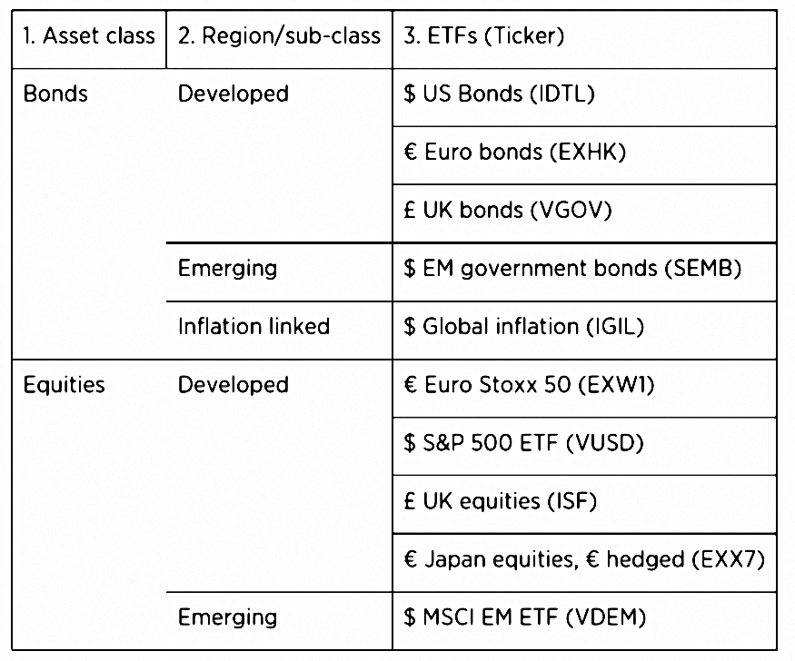
Here are the ETFs that Rob chooses:
He describes a process for working out a volatility target in a series of tables.
He comes up with an annual volatility target of 7.5%
- Using Half-Kelly, that required an SR of 0.15, which he describes as “easily achievable”.
With the maximum after cost SR 0f 0.4, real returns will be 7.5% *0.4 = 3.% pa (“very modest”).
Rob targets a turnover of 0.4 round trips per year with standardised costs of 0.08 SR (which gives 0.4 × 0.08 = 0.032 SR annually).
- With 7.5% annualised volatility that works out to performance drag of 0.032 × 7.5% = 0.24%.
- There are also annual holding costs for ETFs of between 0.05% and 0.55% (say an average of 0.3%).
Correlations and Rebalancing
To work out instrument weights using the hand-crafting method, we need the correlations between the ETFs (Rob provides a table).
- Rob recommends a weekly rebalancing process:
Once again, Rob provides a trading diary which I will pass over.
Systems Trader
In this section, Rob assumes a futures trader with $250K, using the EWMAC and carry rules.
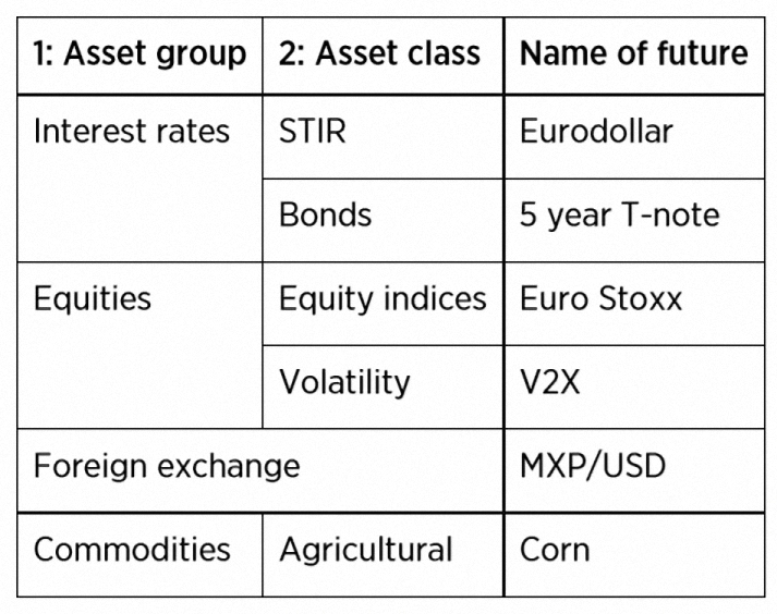
Here is the set of instruments he chooses, based on avoiding large minimum instrument block sizes, low volatility and costs above 0.01 SR:

Trading rules
Rob gets a bit technical here:
Your trend following rules and measures of price volatility will be based on a series of stitched futures prices using the `Panama method’. The optimal calculation requires that you’re not trading the nearest contract, but one further in the future.
This is achievable for volatility (V2TX), Eurodollar and corn. However for the bond, equity and FX future you’ll need to trade the nearest futures contract, as the subsequent deliveries aren’t liquid enough.
Only cheap instruments can trade the fastest rules.
- Rob recommends that you use at least three of the EWMAC varations (so in the worst case scenario, the slowest three).
Now we have four variations across two rules.
Forecast weights
Blending the forecasts from the variations into a combined forecast uses handcrafting.
- The three EWMAC variations are grouped together at the first level.
Rob assumes that all instruments have the costs of the most expensive (V2TX futures – 0.009 SR per round trip).
- The resulting variations in costs (in SR units) are small enough for him not to make any SR adjustments (all SRs are assumed to be equal).
This is the same set of rules that Rob used earlier in the book when combining forecasts, so he already has the answers for the next few steps, including the forecast weights in the table above.
- The diversification multiplier is 1.31
- The middle EWMAC rule has a lower weight because it is more correlated to the other two than they are to each other.
Without correlations, just allocate equally to all three.
Volatility target
Back-testing a system with two trading rules and six instruments from different asset classes, Rob gets an SR of 0.53 (after costs).
- Around 75% of this should be achievable, or SR = 0.40
The rules are mixed between positive and negative skew, and the only negatively-skewed instrument is V2TX, with a 10% weighting.
- So the system has a slightly positive skew.
The volatility target is Half-Kelly, which gives 20%.
- On a $250K portfolio this is $50K.
It’s a relatively high target, and Rob recommends daily checking and adjustments.
Position sizing
To work out price volatility, Rob uses a moving average of daily price changes.
He uses the most expensive instrument (V2TX) to work out whether a longer look-back than the default five weeks can be used.
He also uses the weighted average turnover from the rule variations, which works out at 9.57 round trips per year.
- Multiplying by the diversification multiplier of 1.31 gives a combined forecast turnover of 12.5.
The five-week look back gives a turnover of 12.6, and the 20-week one gives a turnover of 11.7.
- Rob thinks the difference (in turnover, and costs) is too small to justify the slower estimation of price volatility, so he’ll stick with the five-week look back (actually a 36-day EMA).
Costs are 20% * 0.113 = 2.3% on the most expensive instrument.
- There are also charges for rolling over futures contracts, but Rob expects to stay below the “speed limit” of 0.13 SR.
Portfolio
The next step is to set instrument weights by handcrafting (using correlations).
Here are the groups they produce:
Euro Stoxx needs a minimum of 20% weighting because of its large contract size.
- Rob fixes this by increasing the equity allocation to 30% (from a “natural” 20%) to provide headroom.
Process
Rob describes the daily process for a systems trader in a summary table (some or all of this will be automated).
Trading diary
Rob also provides a trading diary, which is a simplified version of what he produces for himself.
Conclusions
And that’s it – we’ve made it through the book.
Today was to an extent a re-run through concepts that we’ve already met in earlier posts.
- But I for one certainly need the practice at this stage.
I’ll back in a few weeks with a summary post describing the key lessons from the whole book.
- Until next time.
Mike Rawson
Mike is the owner of 7 Circles, and a private investor living in London. He has been managing his own money for 40 years, with some success.