Market Timing 2 – Growth & Trend

Today’s post is the second in a series about Market Timing. We’ll be looking at the work of Jesse Livermore on his Philosophical Economics blog.

Philosophical Economics

Philosophical Economics (PhilEcon) is one of the best financial blogs out there, though its format – infrequent and very long, deep posts at irregular intervals – means that it’s not for everyone.

Here’s how the website’s About page describes the content:

Philosophical Thoughts on Macroeconomics, Financial Markets Investing, Accounting, Portfolio Construction, Behavioral Science, Evolution, Game Theory, Pragmatism, Personal Development, and other topics.

It’s written by the pseudonymous Jesse Livermore, named for the famous trader of the 1920s and 1930s.

• The classic book “Reminiscences of a Stock Operator” is about Livermore, and he also wrote a book under his own name.

The original Livermore made a fortune shorting the 1929 crash, but later lost it all and committed suicide in a hotel room.

• The pseudonymous Livermore is very much with us (including on Twitter) and has written four long posts that discuss market timing.

Bad reputation

The first post from Jesse’s that I want to look at is about trend following, but he begins by looking at why market timing has such a bad name.

• People have no issue with diversification across “space” (asset classes).

Market timing is just the same approach across time:

• It divides the time of a portfolio between asset classes according to when they are expected to produce the best returns.

He rejects three reasons why it might be unpopular:

1. trading costs, which are now much lower than historically
2. tax implications, which are mostly a US issue to begin with, and can be avoided by using futures overlays on stock holdings to hedge positions
3. poor timing, since opponents of market timing who believe that markets are efficient must believe that consistently poor timing is as impossible as consistently good timing.

Instead, he thinks there are two other reasons:

• Market timing is about big choices, which lead to stress, which leads to poor outcomes.
• Most market timers have poor investing track records because they stay too long in cash.

Jesse says that market timers are usually cautious types who look for reasons to be out of the market and struggle to get back in.

• He compares this with allocating 95% of a portfolio to cash.

No one would expect anything other than underperformance – but that underperformance wouldn’t discredit the principle of diversification.

Jesse concludes that market timing can add value, particularly when (stock) markets are highly valued, as they are today.

• And he sees the goal of market timing as producing equity-like returns with bond-like volatility.

This is to be achieved by side-stepping downturns.

Trend-following

In the rest of the first post, Jesse backtests three trend-following techniques:

1. simple moving average
   • He uses Meb Faber’s approach which looks at the average of the 10 previous monthly closes – Jesse calls this Monthly Moving Average (MMA).
   • The same approach works with periods from 5 to 50 months, but 10 months works the best.
2. moving average crossover
   • This uses a short MA and a long MA.
3. momentum
   • This compares today’s price to a single value, usually the value from 12 months ago.

These are all binary (in/out, cash/stock, risk asset/safe asset) monthly approaches which produce similar results.

• Note that Jesse uses total return numbers (including dividends), rather than stock price alone – his version of MMA is thus MMA-TR.

Jesse then tests MMA-TR (as a representative strategy) against 235 equity, bond and currency indices, and 120 large-cap (US) stocks.

He uses total return, maximum drawdown and the Sortino ratio to work out whether the strategy has outperformed.

• His conclusion is that the strategy works very well on indices, but very poorly on individual stocks.
• With stocks, trend seems to underperform buy-and-hold 75% of the time.

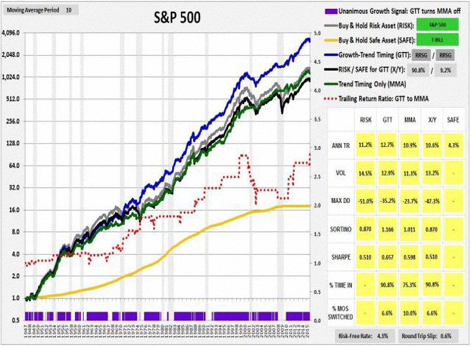
Here are the S&P 500 results:

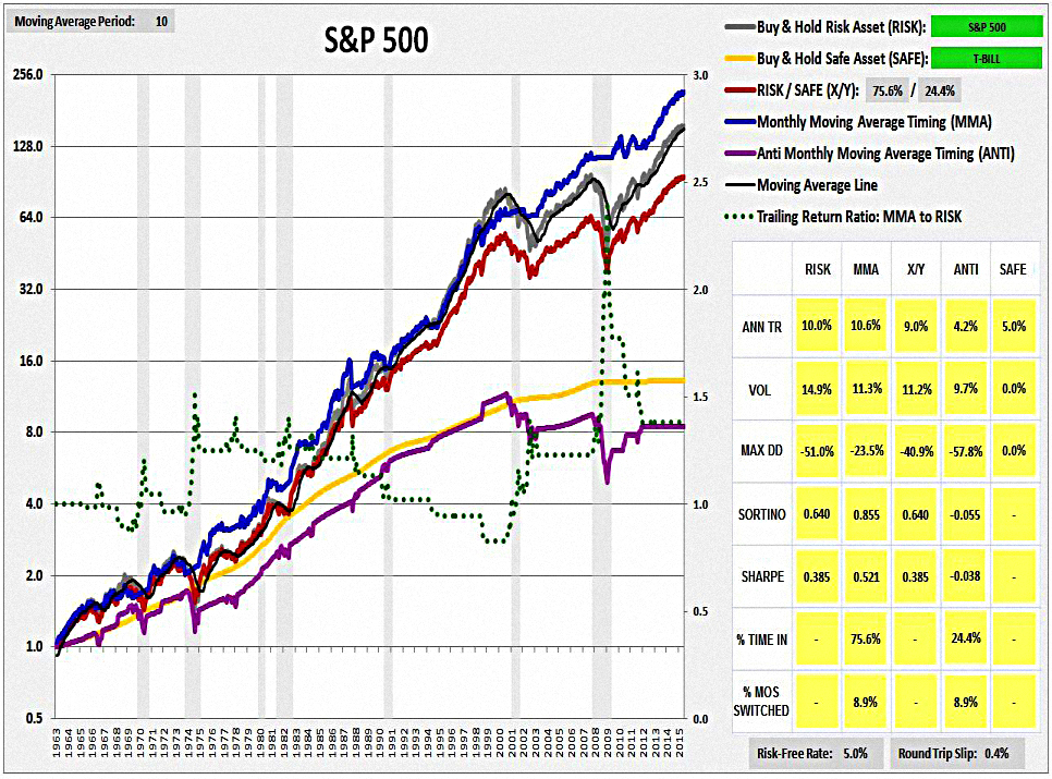
The fact that the strategy performs poorly in individual securities is a significant problem, as it represents a failed out-of-sample test.

Even worse, the traditional explanation of why trend following works should apply to individual securities:

Investors allegedly underreact to new information as it’s introduced, and then overreact to it after it’s been in the system for an extended period of time, creating price patterns that trend-following strategies can exploit. 

---

One factor would be survivorship bias.

• Trend works by protecting against drawdowns, and survivor stocks will be less likely to have had serious drawdowns.
• Jesse notes that the strategy works on “bubble roadkill” failed stocks.

---

He also says that a “stale price” effect will boost the impact of MMA on indices (but not on individual stocks).

• Stocks within an index that do not trade (are illiquid or suspended) will be included in the index at a stale price (from the day before, say).

Momentum trading of indices effectively buys the untraded stock at the stale price, which in an uptrend is likely to be lower than the true price.

• Jesse explained this originally (in an earlier article) in the context of the failed Daily Momentum strategy – which worked until 1999, but then stopped working – but it applies to a lesser extent to MMA.

The stale price effect also explains why momentum performs slightly less well in ETFs (which are tradeable) than in the indices which they track (which include stale prices).

• This effect will be more pronounced with less liquid indices.

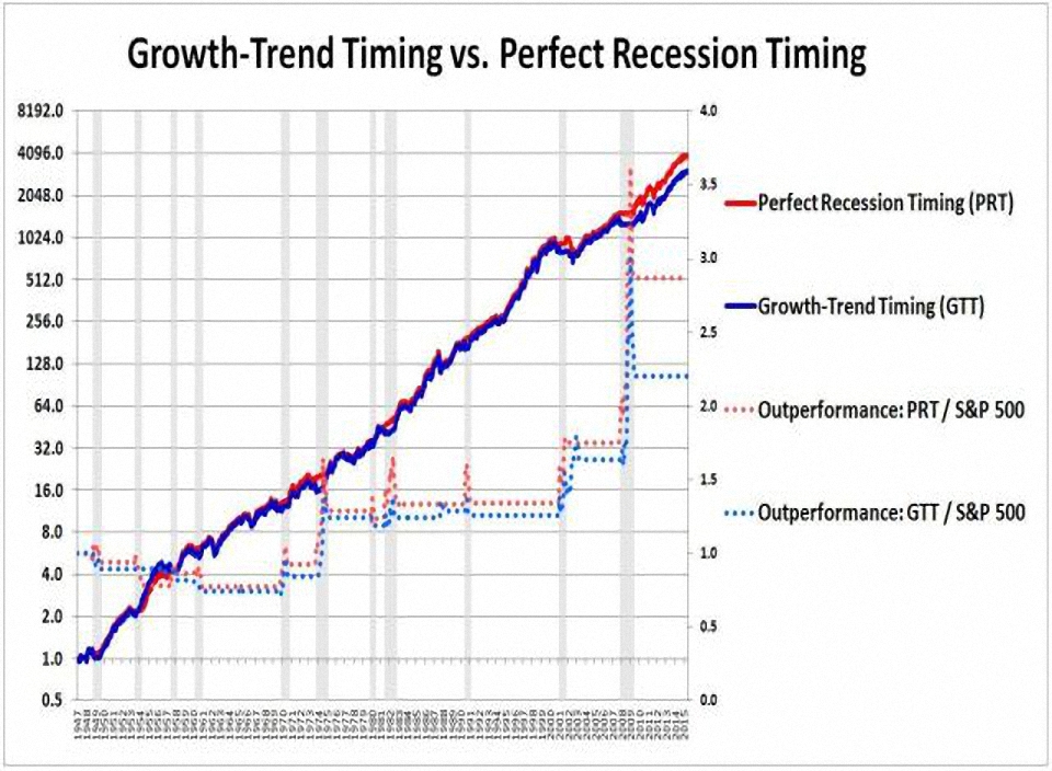
Growth and trend

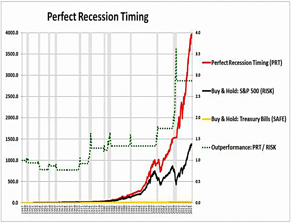
The chart above shows the effect of perfectly timing recessions (selling stocks one month before they begin, and buying back one month after they end).

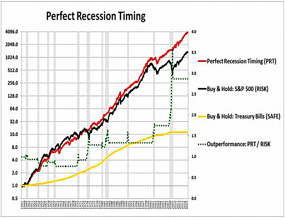
It’s not quite so impressive against a log scale, but it still pretty consistent outperformance.

• Perfect Recession Timing (PRT) generates 12.9% pa, compared with 11.2% from the market.
• Volatility is 12.9% (14.5%) and the max drawdown is 27.2% (51%).

In his third article, Jesse introduces a market timing strategy designed to match PRT by adding a growth filter to the trend-following strategies above.

• He calls this Growth Trend Timing (GTT).

Stop losses

In the next section, Jesse demonstrates how a simple two-way stop-loss rule can be used to capture upside and avoid downside (below the stop value).

• In practice, the assumptions involved (particularly, that of continuous prices) make the model unimplementable in practice.

Price drops can be sudden and skid past our stop.

• Even with continuous checking, there will be price gaps overnight, as well as when new information or large orders hit the market.

Gap losses on each round trip (buy and sell) are the major source of downside for the strategy.

• This is the trade-off for avoiding the downside of the underlying security.
• There is also the bid-ask spread to consider.

Such a strategy performs well against large non-reversing falls, but not against small, self-correcting falls.

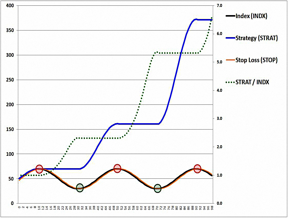
The next section looks at trailing stop losses.

• The three trend-following strategies examined above are all implementation variations of this concept.

Simply using the previous day’s close as the stop works very well, as long as we assume price variations that follow a sine wave pattern.

Downturns and whipsaws

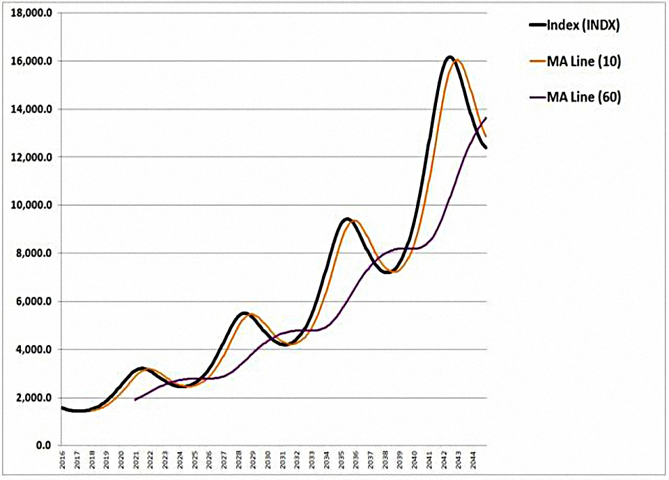
In the next section, Jesse uses an internally retained earnings stream (since he is using total return rather than price) to improve his price model.

• This stream will grow exponentially, in his example at 6% pa.

He adds a sinusoidal valuation wave (PE ratio) from PE = 12 to PE = 20, over a 7-year cycle (to model the business cycle).

• He adds moving averages for 10 months and 60 months.

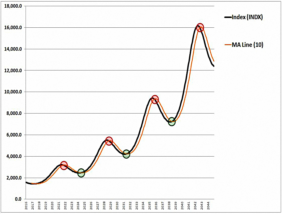
The green dots are buys and the red dots are sells from using the 10-month MA to trade.

• In this model, the 10-month MA outperforms and the 60-month MA underperforms.

Jesse classifies each trade into two types – captured downturns and whipsaws:

• In a captured downturn, the price spends enough time at values below the sale price to pull the moving average down below the (previous) sale price.
• In a whipsaw, the price turns back up above the moving average too quickly.

There’s a simple rule to identify which will happen:

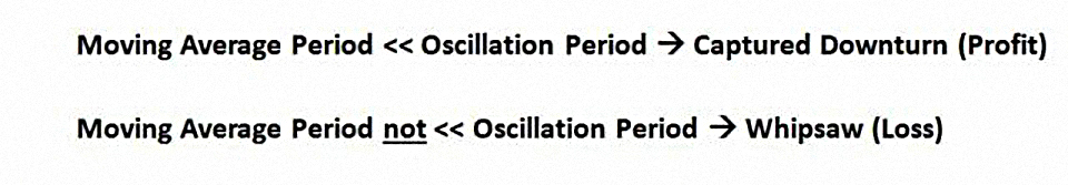
In equities, whipsaws tend to be more frequent than captured downturns, typically by a factor of 3 or 4.  

But, on a per unit basis, the gains of captured downturns tend to be larger than the losses of whipsaws, by an amount sufficient to overcome the increased frequency of whipsaws.

Volatility

The next step is for Jesse to add short-term volatility to both the growth rate and the business cycle sine wave, to get more convincing price data.

• This noise should not, in theory, affect the performance of the trend strategies.

He also adds a 15-month momentum line and a 30 month MA line (the price data is also monthly).

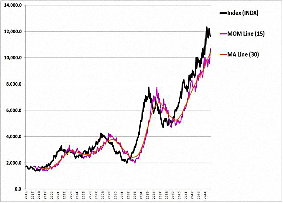
Next he tests the performance of the MA strategy (the cleaner, easier to read line) for various periods.

• As expected, the 20-month MA performs better than the 30-month.
• But the 10-month, 5-month and 1-month are worse, which is unexpected.

The shorter MAs lie closer to the price line, and now that we have a noisy price signal, they pick up more whipsaws.

• Since the “oscillation period” of the noise is very short, the MA cannot be shorter.
• Therefore it must be longer, to avoid touching the price line as much as possible.

---

The second variable to examine is the price checking interval.

• Jesse compares a 5-month MA on monthly price data to a 100-day MA on daily price data.

The results are similar, but on the daily price strategy, the many small whipsaws mean that trading costs (the bid-ask spread) become significant relative to the previously dominant price gaps.

• From 1928 to 2015, the daily version appears to be better.

The problem is that since 1999 it hasn’t worked so well, which could be down to the stale price issue we discussed above.

Indices vs stocks

To work why indices do well with trend strategies, but stocks do not, Jesse looks at each of the elements in his price decomposition in turn.

Higher growth rates impair MMA as there are smaller downturns to avoid.

• But the impact below growth rates of 15% is small.
• High expected growth rates usually occur at market bottoms, and you should be in for the recovery at that stage.

Increasing the amplitude of the cyclicality improves MMA since bigger downturns are avoided.

• Greater short-term volatility reduces MMA performance as discussed above.

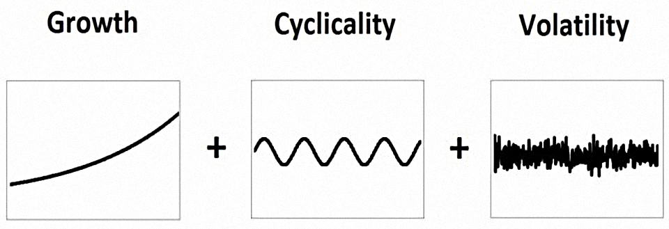
Jesse characterises this as a tug-of-war between cyclicality (large downturns to be avoided) and volatility (lots of whipsaws and bigger gap losses).

• Indexes filter out the volatility of individual stocks whilst preserving their cyclicality, so MMA works better on them.

The volatility comes from the idiosyncratic risks of the individual stocks and the cyclicality comes from the business cycle.

Growth Trend Timing

Jesse believes that the 12-month momentum and 10-month MA strategies work because the periods are short enough to capture the downturns associated with the business cycle.

• There’s no obvious reason why these periods are long enough to avoid whipsaws from noise, but since the strategies work they must presumably be so.

But for the base strategies to continue to work, another large downturn that can be avoided will be required.

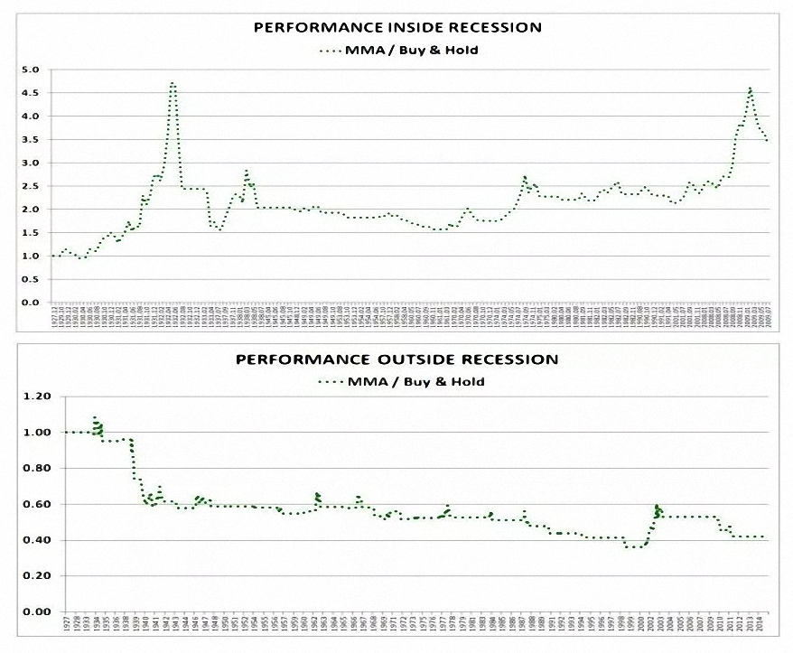
Jesse notes that MMA works well inside recessions, but is not profitable outside of them.

Growth-Trend Timing takes various combinations of high quality monthly coincident recession signals, and directs the moving average strategy to turn itself off during periods when those signals are unanimously disconfirming recession.

That means that when all the signals are positive, the MMA signal is ignored.

• If not, the regular MMA signal is acted upon.

The monthly signals Jesse uses are:

• Real Retail Sales Growth (yoy)
• Industrial Production Growth (yoy)
• Real S&P 500 EPS Growth (yoy, total return)
• Employment Growth (yoy)
• Real Personal Income Growth (yoy)
• Housing Start Growth (yoy)

Jesse normally uses two of the indicators in combination and looks for a unanimous disconfirmation of a recession.

• It might be possible to combine all six indicators to produce a continuous rather than a binary signal.

I’m not sure how many of Jesse’s indicators we’ll be able to find for the UK.

• It might be worth investigating the relationship between UK and US recessions, or perhaps just using the strategy with the US market.

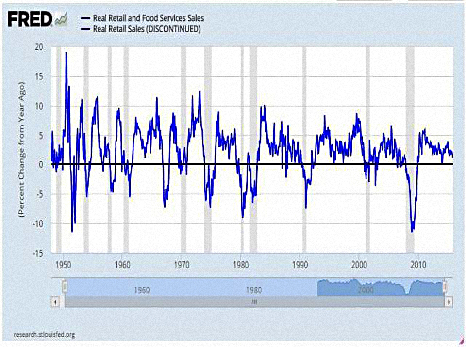
Retail Sales (yoy) is the best US recession indicator.

Here’s how well GTT works using only Retail Sales.

• Jesse’s preferred GTT signal combination is retail sales growth plus industrial production growth.

To prove that the right filters are needed he demonstrates that a Value Trend Timing system (VTT) using the Shiller CAPE adds nothing to the baseline MMA.

Conclusions

1. MMA (and the other trend-following techniques) work for indices but not for stocks.
2. But they work by avoiding large drawdowns, so you need to believe that valuations are high and / or a recession is imminent.
3. Adding recession filters to MMA (to produce GTT) will improve performance when you are not in a recession (or about to enter one).

I’ll be back in a few weeks with more on recession indicators and some reactions to PhilEcon’s GTT model.

• Until next time.