Market Timing 3 – Unemployment and the Taylor Rule

Today’s post is the third in a series about Market Timing. We’ll be looking at the Unemployment Rate and the Taylor Rule.

Last time

Last time out we looked at three very long posts from the pseudonymous Jesse Livermore over at Philosophical Economics.

Our conclusions were:

1. Monthly Moving Average (MMA) – and other trend following techniques- work for indices but not for stocks.
2. They work by avoiding large drawdowns, so you need to believe that valuations are high and / or a recession is imminent.
3. Adding recession filters to MMA (to produce Growth and Trend Timing, or GTT) will improve performance when you are not in a recession (or about to enter one).

The recession filters that Jesse uses (often in combinations of just two) are:

• Real Retail Sales Growth (yoy)
• Industrial Production Growth (yoy)
• Real S&P 500 EPS Growth (yoy, total return)
• Employment Growth (yoy)
• Real Personal Income Growth (yoy)
• Housing Start Growth (yoy)

Today we’re going to look for more recession indicators, and we’ll also look at some reactions to PhilEcon’s GTT model.

Then we’ll move on to the Investing for a Living blog, which has also done a lot of work on market timing.

Perfect recession indicator

The fourth of Jesse’s posts (which we couldn’t fit in last time) is about a particular recession indicator:

• the seasonally-adjusted U.S. civilian unemployment rate (UE)

This is a lagging indicator – high rates occur after a recession has begun.

• But the direction of travel can be a coincident or leading indicator.

The next table shows the lead for turning points in the UE trend versus recession starts:

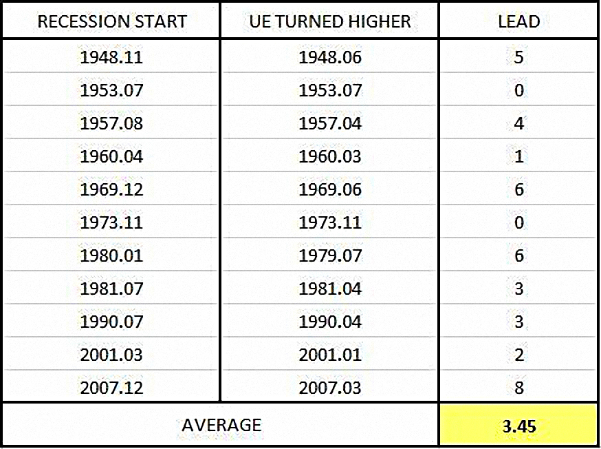
To add more precision, Jesse uses the trailing 12-month MA as a signal:

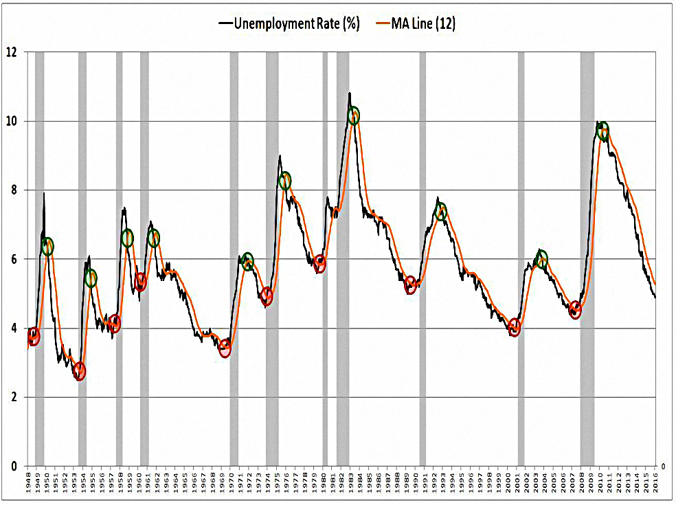
This is a perfect indicator from 1948 to 2016.

• Jesse notes that from 1929 to 1947, the indicator was a little late (for the 1937 and 1945 recessions, not the one in 1929).

It seems these two particular recessions were missed by all the indicators.

---

So now we have seven recession indicators, and the new one is the best:

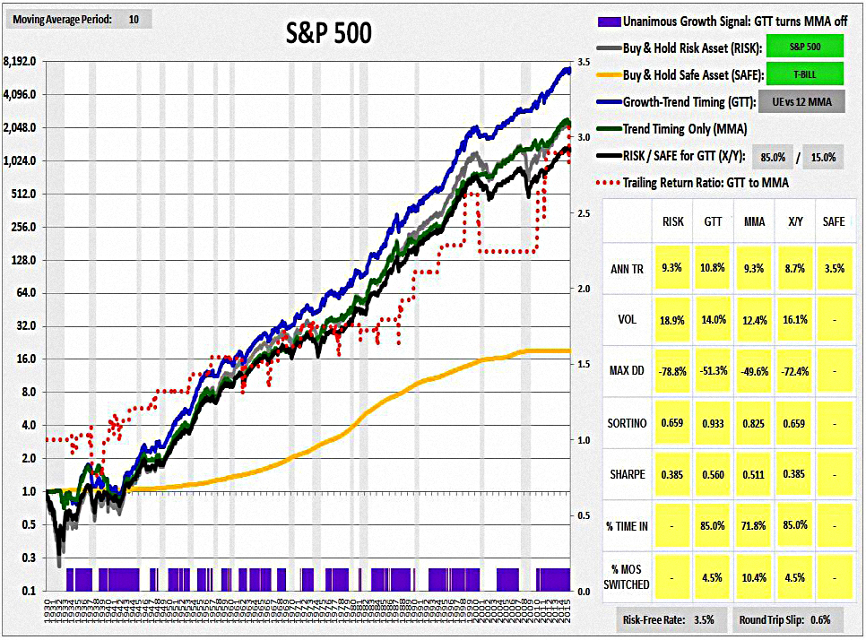
Jesse notes that in a GTT context, we need both the unemployment signal and a downward price trend to get out of stocks.

• The chart shows the performance of such a model.

---

In the same post, Jesse notes that the FRED database used for back-testing includes revised economic data (governments often publish provisional data and then firm it up in subsequent months).

• He demonstrates that using the unrevised unemployment data (as an example) does not affect the GTT signal very much.

This is because the system uses trends and year-on-year comparisons, rather than absolute levels.

---

He also notes a strange result:

If we use U.S. economic data as a filter to time foreign securities, the performance turns out to be excellent.  

But if we use economic data from the foreign countries themselves, then the strategy ends up underperforming a simple unfiltered trend-following strategy.

This is not necessarily bad news, as it will probably be easier even here in the UL to get hold of US economic data.

• But Jesse notes that he needs to look at performance in local currencies in more detail – so this could be partly an FX effect.

As far as I can tell, he hasn’t published this work yet.

Humble student

Around the same time that Jesse was writing his series of posts (back in early 2016), Cam Hui on Humble Student of the Markets published his own piece on the GTT model.

Cam sees three causes of bear markets:

1. War or rebellion causing the permanent loss of capital;
2. Recession; or
3. An overly aggressive central bank tightening monetary policy

GGT only predicts recessions.

Accepting that we won’t have an economic indicator for war, we still need to look out for tight monetary policy.

• He notes that GTT would have stayed long equities through the 1987 crash, when the Fed raised rates twice in the previous month.

Taylor Rule

Cam settles on the Taylor Rule as the best indicator of an overly aggressive monetary policy.

Here’s the Wikipedia definition:

A Taylor rule is a reduced form approximation of the responsiveness of the nominal interest rate, as set by the central bank, to changes in inflation, output, or other economic conditions.

In particular, the rule describes how, for each one-percent increase in inflation, the central bank tends to raise the nominal interest rate by more than one percentage point. 

And here’s the equation:

It’s not an obvious definition:

• i_t is the target short-term nominal interest rate (e.g. the federal funds rate in the US, the Bank of England base rate in the UK)
• π_t is the rate of inflation as measured by the GDP deflator
• π^*_t is the desired rate of inflation,
• r^*_t is the assumed equilibrium real interest rate
• y_t is the logarithm of real GDP, and
• y^~_t is the logarithm of potential output, as determined by a linear trend

Oh, dear – I hope Cam can make this simple for us.

Luckily, he can:

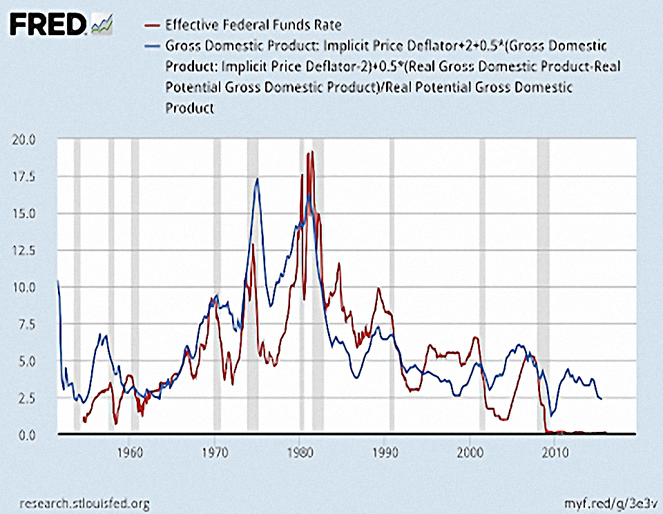
• Cam uses a post from the FRED blog where they use the typical 2% inflation target and a constant 2% real interest rate to generate a Taylor Rule target rate.

Analysis

Cam defines three monetary regimes relative to this Taylor Rule target:

1. Neutral – Fed Funds (FF) within 0.5% of the Taylor Rule target
2. Easy – FF at 0.5% or more below the Taylor Rule target
3. Tight – FF at 0.5% or more above the Taylor Rule target

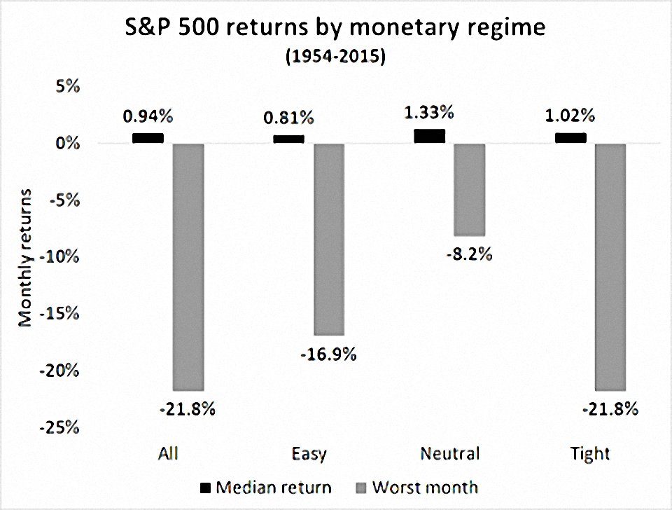
Unfortunately, this first level of analysis doesn’t give us much:

• Monthly returns are higher under a tight regime than a loose one.
• Drawdowns are best under a neutral regime.

The next stage is to look at rising and falling FF rates within each monetary regime.

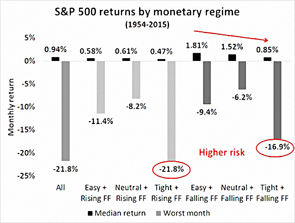
Returns are better when FF is falling, and drawdowns are worse under a tight regime.

• Neatly, returns fall as we move from easy to neutral to tight, even if FF is falling.

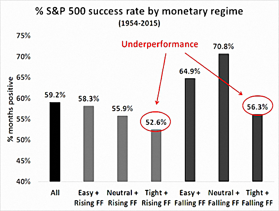
The next chart shows the percentage of positive months, which is much lower under a tight regime – even if the FF is falling.

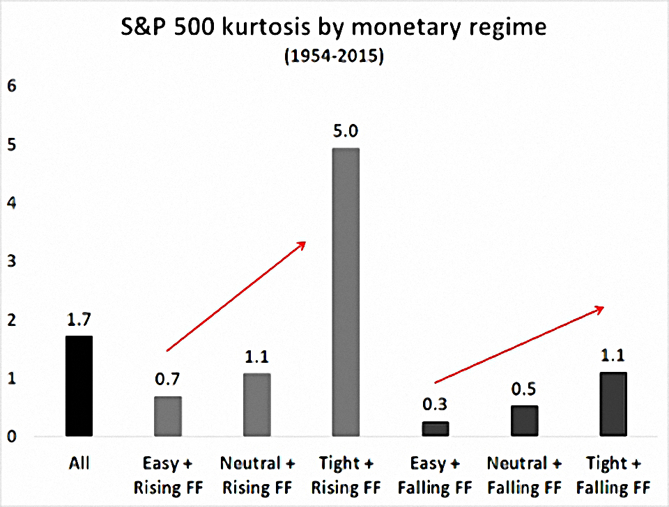
Cam also looked at kurtosis.

• The S&P has fatter tails under a tight regime, especially when the FF rate is rising.

Conclusions

Cam concludes:

• This model is designed for investors who want avoid the kind of large drawdowns that are the result of prolonged bear markets.
• It is definitely not designed to avoid every single 10-20% correction that comes along. Even under neutral and easy monetary regimes, single month drawdowns of about 10% can and do occur.
• Equity investors have to be able to accept those kinds of risks, as they just come with the territory. Otherwise if you can’t stand the heat, stay out of the kitchen.

1. We’ve added a new recession indicator, which is better than the six we already had.
2. And we’ve learned how to avoid bear markets cause by excessively tight monetary policy.

I think we can figure out how to avoid bears caused by war on our own.

---

In the next article, we’ll look at the timing model put together by the Investing for a Living blog.

Until next time.