Smart Portfolios 2 – Uncertainty and Optimisation
Today’s post is our second visit to Rob Carver’s book Smart Portfolios.
Contents
Uncertainty

Chapter Two of Rob’s book is about uncertainty, and how you can use what happened in the past to make predictions about the future.
Rob makes no distinction between investing, trading and gambling since they all involve risking money with an uncertain outcome.
- The big mistakes are betting when you will lose on average (no edge/odds against you) and putting too much money into a single bet.
- The key is betting more when the odds are in your favour.
Rob imagines investment as a game with a very large deck of cards whose contents are not known.
- Each card has a number which indicates an annual return – some of which are negative.
- Each round (year) you need to decide how much to bet (or not to bet at all).
So we need to predict the value of the next card, based on a model which includes an expected average and some measure of the variation in the outcome (volatility, sometimes called risk).
- The advantage of the investment game over blackjack is that we can see all the cards that have already been dealt.
- The disadvantage is that this doesn’t tell us which cards are left in the deck.
Rob assumes that with a deck of infinite size (infinite possibilities), the remaining cards will look like the ones that have already been dealt.
- In other words, past performance is a guide to the future – the opposite of what the regulatory warnings say.
In investment, more good cards already played means more good cards to come.
Statistics
To decide whether to play, you need to know the expected average return, which needs to be positive.
- You also need to know the volatility of returns, for which Rob uses the standard deviation.
Equities return around 5% to 6% pa, with a standard deviation of 25% to 30%.
- Bonds have lower returns, with SDs of 1.5% (short government bond) to 8% (10-year).
Most analysis assumes Gaussian (normal) returns since you only need the mead and SD to define this distribution.
- This means that returns should be within one SD on 68% of occasions, and within two SD on 95% of occasions.
In reality, stock returns, in particular, have fat tails – extreme results are more common than would be expected.
With a Gaussian distribution you’d get a 4 standard deviation fall on only 1 out of 31,500 days (roughly once every century). But from 1914 to 2014 the Dow Jones Index had a 4 standard deviation fall on more than 30 occasions!
You also need to know how uncertain you are about your estimate of the geometric mean (and therefore how likely it is that is really is positive).
- Rob approaches this via “bootstrapping” – constructing “alternative histories” from the real historical data.
It sounds a bit like Monte Carlo analysis to me.
- Rob works out a distribution of mean returns from the alternative histories.
From this, he can work out the change that the “true mean” is above zero.
Optimisation
Rob is not a great believer in the standard portfolio optimisation techniques.
- Because they are usually applied to returns from the recent past, they often lead to extreme weightings.
Instead, Rob works from a list of assets to find the portfolio with the best returns for a given level of volatility (SD, or “risk”).
He starts with the classic stocks and bonds portfolio.
- Equities have higher returns, so they are good.
- Bonds have lower risk, so they are good, too.
To work out the best mix, Rob uses the Sharpe Ratio (SR), which measures returns per unit risk (volatility).
- As we know, diversification (the combination of non-correlated assets) lowers risk and so will increase SR.
To simplify the maths, Rob does not subtract the (currently historically low) risk-free return from the asset return before calculating the SR. (( He also assumes for most of the book that all assets have the same SR, and in the final part uses only relative SRs ))
- The US 10-year Treasury returns 1.9% pa with a volatility of 8.27% for an SR of 0.225
- The S&P 500 returns 6.2% with a volatility of 19.8% for an SR of 0.315
Returns fall as bonds are added to stocks.
- Volatility also falls, but the low point uses less than 100% bonds (because of diversification).
The SR increases until around 65% bonds – but 100% bonds are worse than 100% stocks.
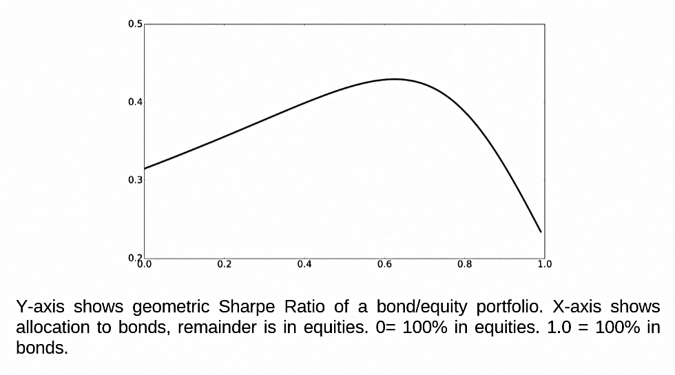
So the best portfolio is not obvious:

Some people might want the highest SR, but others (including me) will want a higher return than that.
- But everyone should want a portfolio somewhere along this efficient frontier.
Example portfolios
In the next section, Rob runs through some imaginary portfolios with imaginary assets.
- Portfolio 1 has three almost identical assets with high correlations, and the optimal portfolio is an even split.
- Portfolio 2 has identical assets with no correlation and is also split evenly.
- Portfolio 3 has an uncorrelated asset and two highly correlated ones.
- The uncorrelated asset picks up almost half of the total cash, with the rest split between the other two.
- Portfolio 4 has uncorrelated assets, one of which has higher volatility.
- The allocation to this asset is lower, but Rob is uncomfortable that it’s hard to see how much lower it should be.
- Portfolio 5 has highly correlated assets with one slightly riskier.
- This riskier asset now gets a zero weighting!
- Portfolio 6 has highly correlated assets, one of which has a slightly higher return.
- Now the entire portfolio is in that asset!
- Portfolio 7 has uncorrelated assets, one with a much higher return.
- Now the weights change almost in proportion to the returns.
We can see those small variations between highly correlated assets lead to massive changes in weightings.
- But this “tipping point” problem is not so large with uncorrelated assets.
Unstable portfolios
In the next section, Rob repeats the bootstrapping exercise he carried out to calculate the uncertainty of the historical mean.
- This time he looks at standard deviation, correlation and the Sharpe Ratio.
The variation in means between bonds and equities is many times larger than the small (0.5%) difference in means that can produce extreme portfolio weights.
Standard deviations (volatilities) are less uncertain, and we can be confident that stocks are riskier than bonds (the distributions don’t overlap).
- We should be less confident that the higher mean compensates for the higher volatility.
Correlations also have less uncertainty than means.
Most importantly, it’s almost impossible to distinguish between the historic Sharpe ratios of stocks and bonds.
- The average SR is around 0.2
The key problem that this throws up is that standard optimisation techniques can produce a wide range of allocations to equities.
- Things would be even more volatile with assets more highly correlated than stocks and bonds.
Rob has three ways of dealing with this:
- risk-weighting
- the “hand-crafting” process (which we will meet later)
- an assumption that risk-adjusted returns (SRs) are identical for all assets.
Lower future returns
Like me, Rob believes that future returns for most asset classes will be lower than previously.
- Low inflation means than nominal returns will be lower, but real returns will also be lower.
Over the past 30 to 40 years, falling inflation led to lower interest rates.
- This meant higher bond prices and higher PEs for stocks.
Any return of inflation would see the process reverse.
Note that with low returns, costs become very important.
Rob provides his own adjusted expected future returns – he’s going for 3% real for equities, with an SR of 0.15.
- I think this is plausible, but it’s also problematic.
It’s below our failsafe SWR of 3.25% pa (and that retirement portfolio is only 75% equities).
- Given that the SWR is derived from historical data, I think that Rob’s approach may have ignored the sequencing effects in equity returns.
We are not quite at historic highs, so there’s no reason to expect historically low future returns.
- Or it could be that the SWR includes the fallback option of running down your capital over 40+ years, in the event that returns are lower than required.
I think that real equity returns could be as high as 4% pa over the long-term, but I wouldn’t be shocked if Rob turns out to be right and not me
- Or if returns were even lower than Rob thinks.
Rob’s adjusted numbers produce a max SR portfolio that is 68% bonds and 32% equities.
- This is far from any portfolio that I would ever hold.
The SWR retirement portfolio (max long-term returns) is 75% equities.
- Note that Rob’s allocation is for a US-only portfolio.
- International diversification will lower risk and support higher equity allocations.
Conclusions
It’s been another interesting visit to Rob’s book.
I’m especially pleased to discover that portfolio optimisation doesn’t work in practice.
- I’ve been using my own version of “hand-crafting” asset allocations for decades.
I hadn’t realised that SRs are broadly equivalent across assets, but then I have my doubts about SR:
- it includes upside volatility (or rather, it counts it as bad rather than good), and
- more importantly, I don’t want the max SR portfolio.
I want the highest returns for the level of volatility than I can tolerate.
- Sortino is a better measure, but less easy to calculate (and so less often calculated).
We’ve also learned that historic (relative) volatility and (relative) correlations are broadly reliable.
Until next time.
Mike Rawson
Mike is the owner of 7 Circles, and a private investor living in London. He has been managing his own money for 40 years, with some success.