The Optimal Stack

Today’s post is about a recent article from NewFound and ReSolve about the best possible stacked portfolio.

Stacking

NewFound and ReSolve (together known as Return Stacked Portfolio Solutions, or RS) are some of the biggest proponents of stacked portfolios (also known as portable alpha, or to me and you, plain old leverage).

• They offer a range of ETFs with total allocations greater than 100%, and I will be surprised if the study doesn’t come up with a result that can be constructed from their range.
• Unfortunately, I can’t buy these ETFs here in the UK, so today will be a theoretical exercise for me.

The Optimiser

RS say that advisors ask them a lot what the optimal stack is.

To answer the question, they start with a portfolio optimiser, running 10,000 25-year histories (2000 to 2025) across five asset classes (U.S. stocks, U.S. bonds, gold, managed futures, and merger arbitrage).

• Merger arbitrage will be hard to access in the UK.

RS say that the optimum portfolio (at the same volatility as the traditional 60/40) is weird and would be hard to stick to (I’m guessing in part because of large tracking error against the 60/40).

Instead, they recommend diversifying across multiple strategies.

• This gives comparable risk-adjusted returns with much less behavioural pain.

The note looks at different blending approaches in order to help investors (and advisors) come up with a stack that can be held for 20 years.

But first, the optimiser.

• RS adjusted the Sharpe’s of the asset down from their historical values.

Historical Sharpe ratios over this period were unusually high for several asset classes, driven by favorable macro tailwinds, sample-specific mean reversion, and the general tendency for realized returns to exceed ex-ante risk premia over any finite sample. 

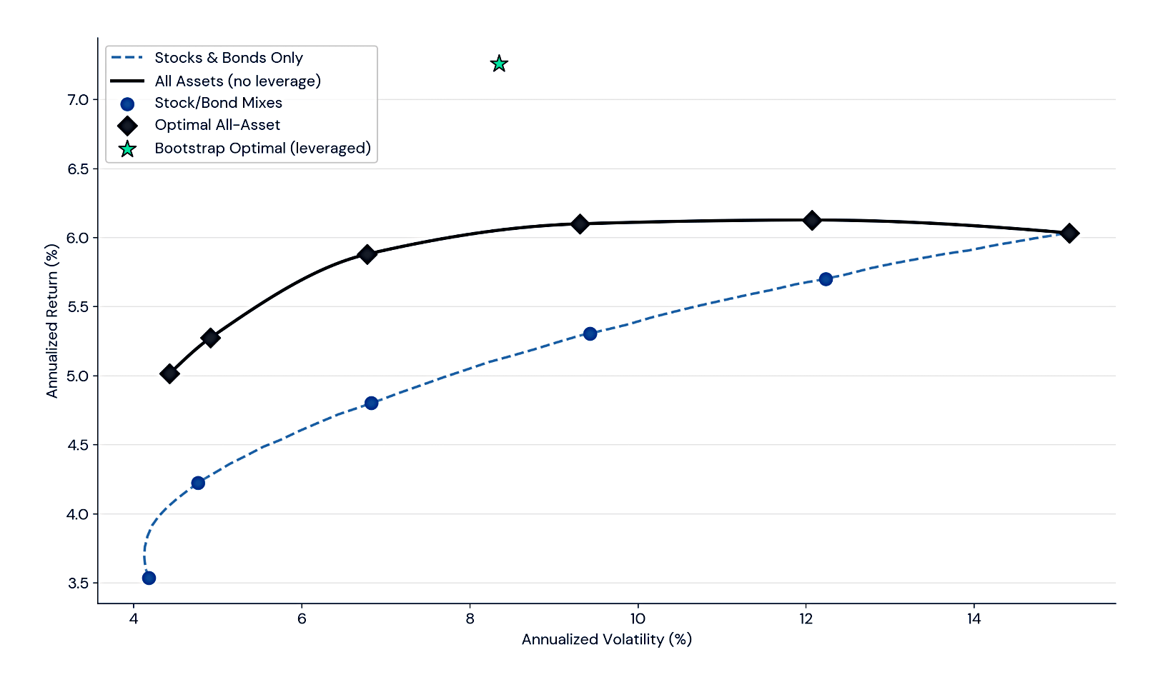
Across the 10,000 simulated histories, the bootstrap-optimal portfolio produced a median return of 7.3% at a mean volatility of 8.3%, meaningfully above the 60/40’s 5.3% at 9.4% volatility.

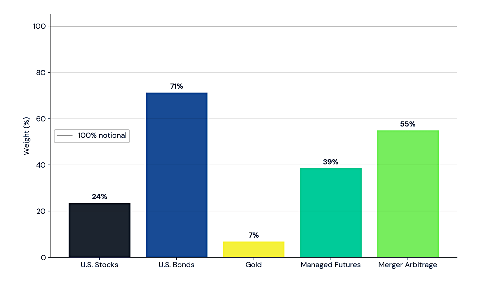
Twenty-four per cent in stocks. Seventy-one per cent in bonds. Thirty-nine per cent in managed futures. Fifty-five per cent in merger arbitrage. Total notional exposure of 195%.

That’s quite the portfolio, and a long way from 60/40 (although it matches for volatility). 

While recent returns may look weak, that backwards-looking disappointment is largely a reflection of rising yields, which can be good news for future returns. 

When yields rise, they simply reallocate return from the present into the future, and when they fall, they pull some of that future return forward.

Behavioural roller coaster

The optimal portfolio has a tracking error of 7.8% relative to a 60/40. Over any given 12-month period, the return difference between this portfolio and a 60/40 ranged from −17 percentage points to +32 percentage points.

In roughly half of all rolling 12-month windows, the optimal portfolio trailed a 60/40, and nearly one in three periods saw underperformance exceeding five percentage points.

As you would expect, the outperformance comes when stocks are struggling, and the underperformance comes during stock rallies.

The optimal portfolio essentially matched the 60/40 over the post-2009 bull market, holding only 24% in stocks during one of the greatest equity runs in history.

A great result, but a path that would be difficult to explain to a client (or to stick to as a DIY investor).

Tracking error

A three-year stretch of underperformance is a rounding error in a Monte Carlo simulation; it can feel like a lifetime in a quarterly review. Tracking error turns out to be one of the most useful frameworks for calibrating how much to stack.

Tracking error is the deviation from the benchmark. 

• In traditional portfolios, diversifiers replace the return of stocks or the stability of bonds, but in return stacking, diversifiers can be added to the strategic asset allocation (SAA).
• In particular, the equity-bond split can be matched to risk tolerance (and time horizon, etc.).

The diversifier overlay becomes the sole source of tracking error. In our experience, roughly 2–3% annualized tracking error is the upper bound of what most clients can tolerate over a full market cycle. 

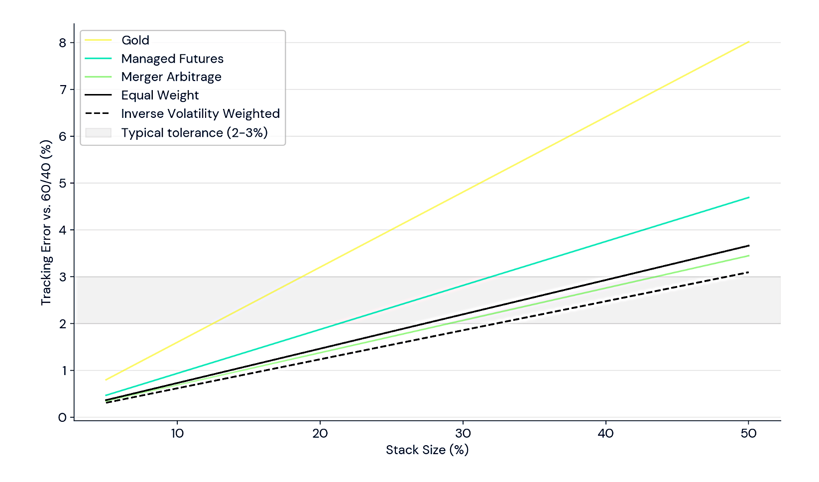
How much you can fit within a 2% tracking error budget (per risk budgets) depends on what you are stacking.

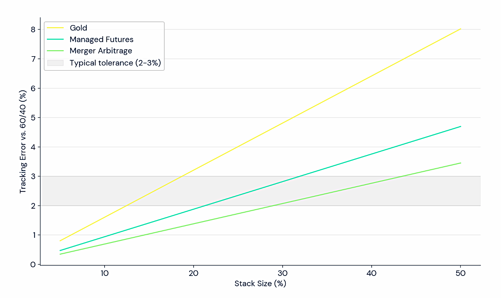
The tracking error scales with the volatility of the diversifiers.

Gold, with an annualized volatility of 16%, hits the 2% tracking error threshold at roughly a 12% stack size. Merger arbitrage, at 7% volatility, doesn’t reach 2% tracking error until nearly 28%.

As with unstacked portfolios, you need high volatility diversifiers at small allocations.

A 5% allocation to merger arbitrage generates roughly 0.3% of tracking error, barely distinguishable from noise. That same 5% in gold generates roughly 0.8%. Neither is likely to materially improve portfolio outcomes.

Diversify Your Diversifiers

You can get more bang for your buck by blending diversifiers.

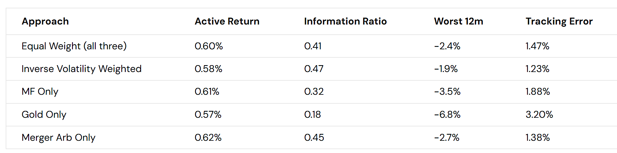
The diversified blends deliver information ratios (active return per unit of tracking error — a measure of how efficiently a strategy converts its deviation from the benchmark into excess return) comparable to the best single-diversifier approach, without requiring the allocator to identify that best approach in advance.

The Inverse Volatility Weighted approach’s average worst-case 12-month shortfall was just 1.9 percentage points. The single-diversifier approaches had average worst-case shortfalls of 2.7–6.8 percentage points.

Diversification also enables a larger stack within the same tracking error budget. The same behavioral tolerance that limits single-diversifier stacks to 10–15% may permit a blended stack of 20–25%.

This is a fancy way of showing that the diversifiers have low correlations with each other, not just with stocks and bonds.

We see most allocators landing between 10% and 25% total stack, using two to three diversifiers.

That’s the approach that I’m moving towards personally, insofar as the constraints of UK tax shelters will allow.

Implementation

If we blend through equal weighting, we are implicitly tilting toward higher-volatility diversifiers.

• This can be OK, but it means more tracking error (and a smaller stack).

One fix is inverse volatility risk weighting (as per Risk Parity).

Weights are computed using each diversifier’s trailing 36-month volatility and updated monthly.

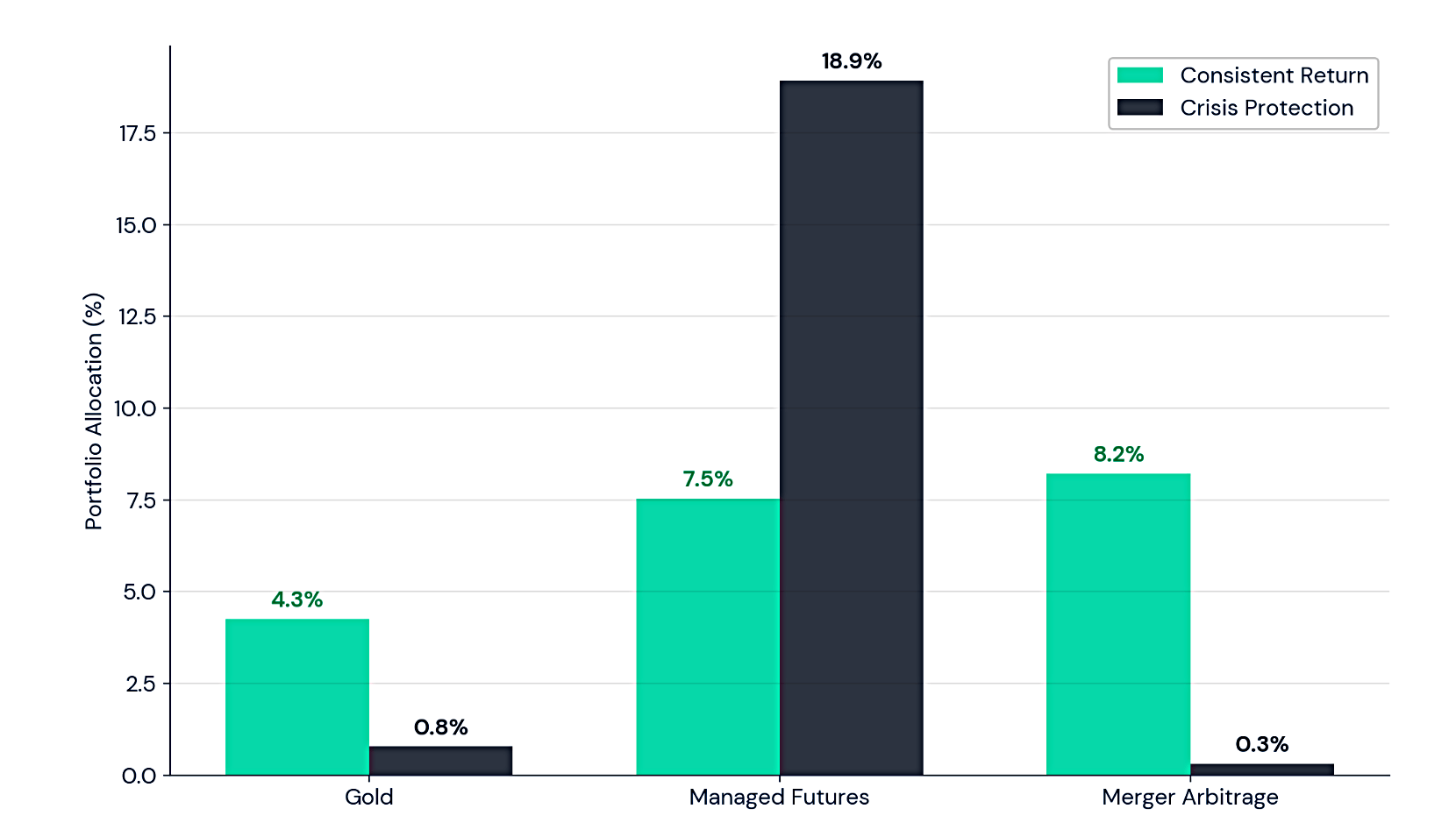
Two more options are to weight for consistent returns, or for maximum drawdown (crisis protection).

• For consistency, RS uses the percentage of rolling 12-month windows where the stacked portfolio outperforms the benchmark.

The optimizer lands on a blend of 21% gold, 38% managed futures, 41% merger arbitrage. That translates to 4.3% gold, 7.5% managed futures, and 8.2% merger arbitrage [in a 20% stack overlay].

The mini-max drawdown portfolio is quite different:

4% gold, 95% managed futures, 2% merger arbitrage. In portfolio terms: 0.8% gold, 18.9% managed futures, and 0.3% merger arbitrage. 

This blend improved the 60/40’s max drawdown by 3.4 percentage points on average, but the median excess return was only 0.66 percentage points, and the blend was positive in just 61% of 12-month windows.

The big takeaway here is that managed futures are great for crash protection.

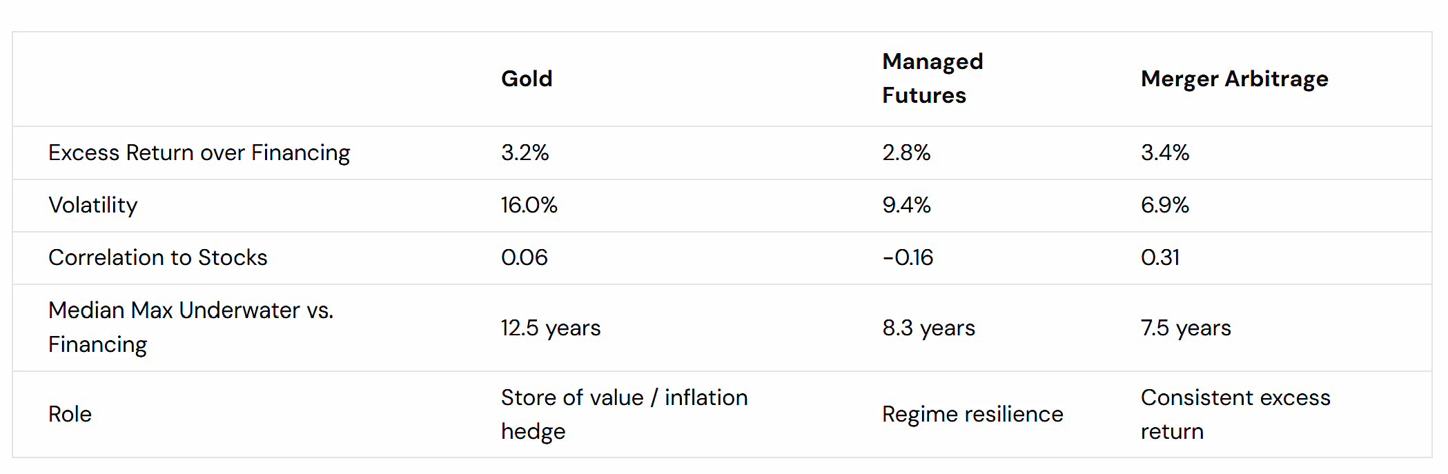
RS characterise diversifiers as either defense or offense.

• Manager futures and gold have low correlations to stocks and do well when stocks are struggling.
• The cost of this is years of underperformance.

Merger arbitrage has more consistent returns but a higher correlation to stocks.

Conclusions

The main takeaway from today is that there is no optimal stack – you need to figure out which best fits your needs, so that you can stick with it.

• We also learned that we need to diversify our diversifiers, and that trend is good in a stock market crisis.
• With a good blend of diversifiers, a 25% stack should be possible without drifting too far from your underlying SAA.

That’s a reasonable target to aim for, but with my portfolio constraints, the RS lower bound of a 10% stack feels more realistic.

---

That’s it for today.

• Until next time.