Tail Risk Protection

Today’s post looks at some non-intuitive ideas around tail risk protection.

Mike Lawler

Today’s post is inspired by a Twitter thread from Mike Lawler (@mikeandallie).

• I hadn’t come across Mike before, but his thread was retweeted into my feed by someone that I do follow.

Mike describes himself as a former maths professor.

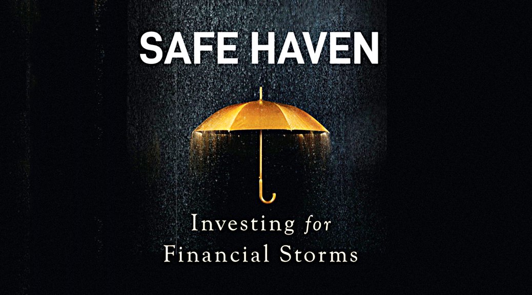
He had just finished reading Mark Spitznagel’s recent book, Safe Haven.

• Mark is a friend and former colleague of Nassim Taleb and takes Taleb’s ideas around barbell portfolios to extremes.

I haven’t read Safe Haven yet, but I have read Mark’s earlier book, The Dao of Capital.

I found it very interesting on a philosophical level, but short on practical advice as to how to implement its key ideas.

• I’ve heard similar things about the newer book.

Mike’s takeaway from Safe Haven was that buying crash protection can increase your expected return, even if you pay above the cost of loss.

The game

To illustrate the concept, Mike imagines a game with the following rules:

• 50% of the time your wealth increases by 10%
• 30% of the time your wealth increases by 5%
• 10% of the time your wealth is unchanged
• 9% of the time your wealth goes down by 5%
• 1% of the time your wealth goes down by 80%

This has an expected return of 4.25% pa, but with quite a wide spread.

• The chart shows 100K simulations of running the game for 100 turns.

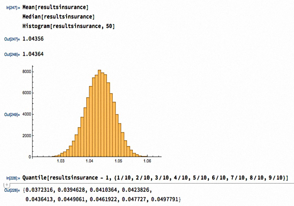
The second version of the game introduces insurance for the 1% worst case – an 80% loss.

• The insurance costs 1.6% and only pays out in the down 80% year.

The rules of this new game are:

• 50% of the time your wealth increases by 8.4%
• 30% of the time your wealth increases by 3.4%
• 10% of the time your wealth goes down by 1.6%
• 9% of the time your wealth goes down by 6.6%
• 1% of the time your wealth is unchanged

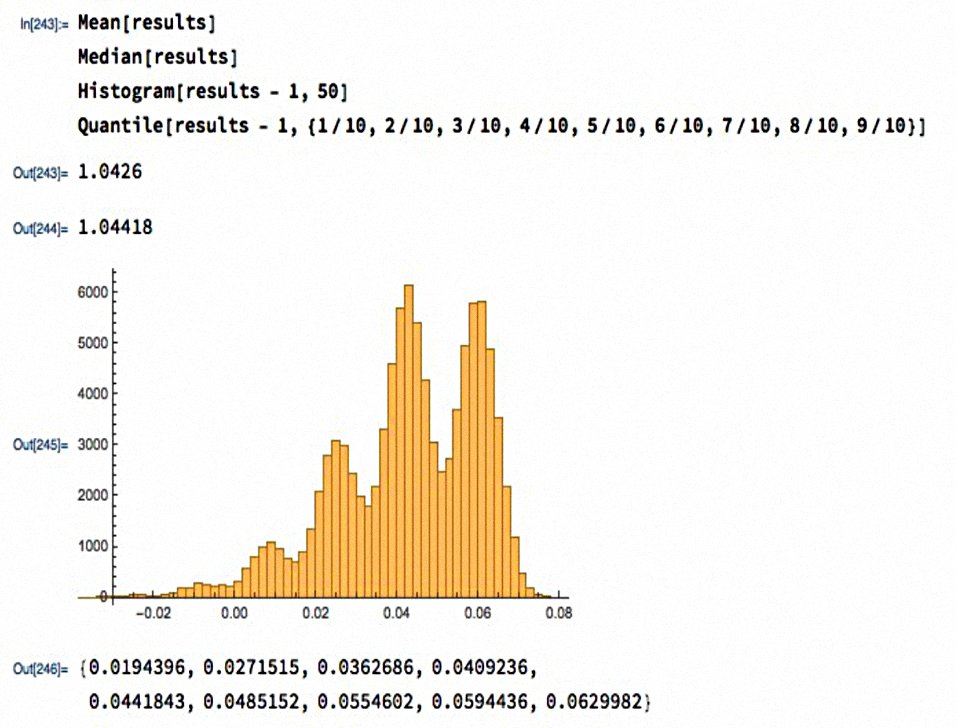
The surprising result is that the average return from 100 runs is now 4.35% rather than 4.25%.

• That’s despite the fact that the insurance costs 1.6% and the expected value of the insured loss is only 0.8% (1% * 80%).

We also have a much tighter spread of outcomes, which looks more like a normal distribution.

• We’ve given up the very best outcomes and avoided the very worst ones to produce a slightly better average result.

Mike says:

The book shows details of a bunch of examples like this – also without any heavy math at all, really just arithmetic. Spitznagel’s book is an interesting read. It isn’t technical at all.

This was a pretty good thread, and it naturally provoked some responses.

Benn Eifert

One of the best came from Benn Eifert (@bennpeifert), who is someone I do follow on Twitter.

• Benn is a derivatives guy.

He linked to an old thread of his from 2021, which I had saved at the time.

• The starting point for his thread was this idea:

We are long-term investors. Volatility doesn’t matter to our portfolio.

This sounds good, but unfortunately, volatility reduces the long-term compound growth rate (CAGR) of a portfolio.

• This effect is called variance drag.

Let’s consider two return streams, both with average annual returns of 10%, but with annualized volatility of 10% and 20% respectively. The long-term compound growth rates of the two portfolios will be 9.5% and 8.0%!

The loss from volatility is half the variance (which means half the square of the volatility).

A reduction in volatility from 20% to 10% for the same average annual return increases the long-term compound rate of growth by 150 basis points.

And if volatility is high enough, compound returns will go negative.

This concept is related to the idea that if a portfolio loses 50%, it needs a 100% gain to get back where it started, not just a 50% gain.

Tail hedging

Benn moves on to the popular view on tail hedging:

Tail hedging involves buying option-based insurance against market drawdowns. Because markets generally charge a risk premium for insurance, the expected returns of a tail hedging strategy over long periods of time are negative.

As a result, along-term-oriented asset owner should not allocate to hedging strategies, as they will detract from long-term compound returns.

The idea that tail hedging should produce negative long-term expected returns (as per Mike’s insurance) is fine.

Individual long convexity trades at certain points in time may be mispriced and smart, dynamic hedging strategies might be able to reduce the cost of carry over time, but it is unrealistically optimistic to think that tail risk hedges can make money systematically over time.

But that doesn’t mean that tail risk hedging doesn’t work.

Tail risk hedges are inversely correlated with the performance of risk assets and produce outsized returns during times of crisis. If tail risk hedges are added to a long-term, regularly rebalanced portfolio, they can cushion drawdowns and mitigate the mechanical reduction of risk asset exposure during times of stress.

In doing so, they can enhance the long-term compound rate of return of the overall investment program, despite the hedges themselves losing money over long periods of time on a stand-alone basis.

The crisis alpha from the tail hedge means more exposure to risk assets just after a crash (which is usually a good time to be invested).

Systematic hedge

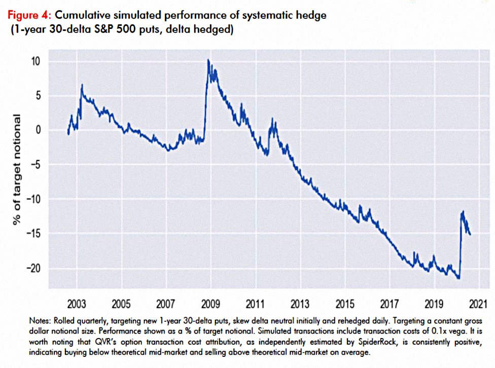
To illustrate, Benn looks at a hedging strategy he describes as “nothing special” – 1-year 30-delta puts, delta hedged and rolled quarterly.

• This loses money as a stand-alone strategy.

But if this strategy is added to a 60/40 portfolio, you get lower volatility and higher returns.

As Benn says:

Many do not understand this.

Hawk & Serpent

We also came across this idea when we looked at Chris Cole’s Hawk and Serpent paper, and the underlying Dragon portfolio.

• The chart above was also referenced in the Twitter thread.

The paper looks at combining a high-return asset (A) with either a lower-return asset (B) or an asset with slightly negative returns, but a negative correlation (C).

• Paradoxically, A+C generates the same returns as A+B with much lower volatility.

This means that with leverage, you can increase the volatility of A+C to match that of A+B and receive much higher returns.

• This is the principle underlying risk parity portfolios.

---

That’s it for today.

• Correlations work in mysterious ways.

Until next time.