How much Trend? – Carver

Today’s post looks at an article from last year by Robert Carver on how much trend we should have in our portfolios.

Rob Carver

Robert Carver is one of my favourite authors and financial commentators.

• He’s written three books (with a fourth due later this month), each of which we have analysed on this website.

Smart Portfolios in particular had a huge influence on the way I structure the passive portfolio that forms the core of my investment strategy (with a 35% allocation).

• To be fair, I was using a similar approach before I read the book, but Rob helped me to improve and refine the portfolio, as well as providing mathematical explanations for why it’s a good idea.

The other two books are also great, but they steer you towards trading futures, and I don’t have enough money outside of UK tax shelters to implement Rob’s system.

• His trading system is open source and under constant development, and anyone with enough spare capital can use it.

How much trend?

This is a surprisingly hard question to answer.

• I’ve heard anything from a 10% allocation to trend to 60% trend, but I’ve never seen an analysis to support either of these figures or any number in between.

Here’s Rob’s opener on the subject, from his blog post entitled “Optimal trend following allocation under conditions of uncertainty and without secular trends”:

Few people are brave enough to put their entire net worth into a CTA fund or home grown trend following strategy (my fellow co-host on the TTU podcast, Jerry Parker, being an honorable exception with his ‘Trend following plus nothing’ portfolio allocation strategy).

Although Rob has become known as a trend follower (probably through his regular appearances on the Top Traders Unplugged podcast), in practice his system uses lots of rules and is perhaps only two-thirds trend.

• Rob has also stated several times that most of his money is in a passive ETF portfolio and in some UK dividend stocks.

So Rob’s allocation to trend is probably in the 20% to 30% area.

• He says that he wouldn’t be able to tolerate the daily fluctuations in portfolio value if he was 100% trend and that he prefers regular income to fund his living expenses.

Rob’s 25% (say) is still a chunky allocation for a UK private investor.

• As mentioned above, I struggle because I haven’t found a way to access trend from within UK tax shelters (SIPPs and ISAs).

There are useful ETFs in the US, but none over here.

• So my manual, taxable allocation is much lower than Rob’s (and, I expect to find today, much lower than optimal).

Historical returns

Rob warns against using (recent) historical returns, as he does in Smart Portfolios: (( Very long-term returns, particularly between asset classes, such as stocks return more than bonds, do factor into his final portfolio design ))

1. Standard portfolio optimisation techniques are not very robust
2. We often assume normal distributions, but financial returns are famously abnormal
3. There is uncertainty in the parameter estimates we make from the data
4. Past returns distributions may be biased and unlikely to repeat in the future

He gives as an example the excellent returns from stocks and in particular bonds as interest rates and inflation (and equity discount rates) have fallen since the 1980s.

• We can’t expect these conditions to continue, and we don’t want to design a portfolio that assumes that they will.

Skew is also a complicating factor since stocks have negative skew (long left tails) and trend has a positive skew.

The assets

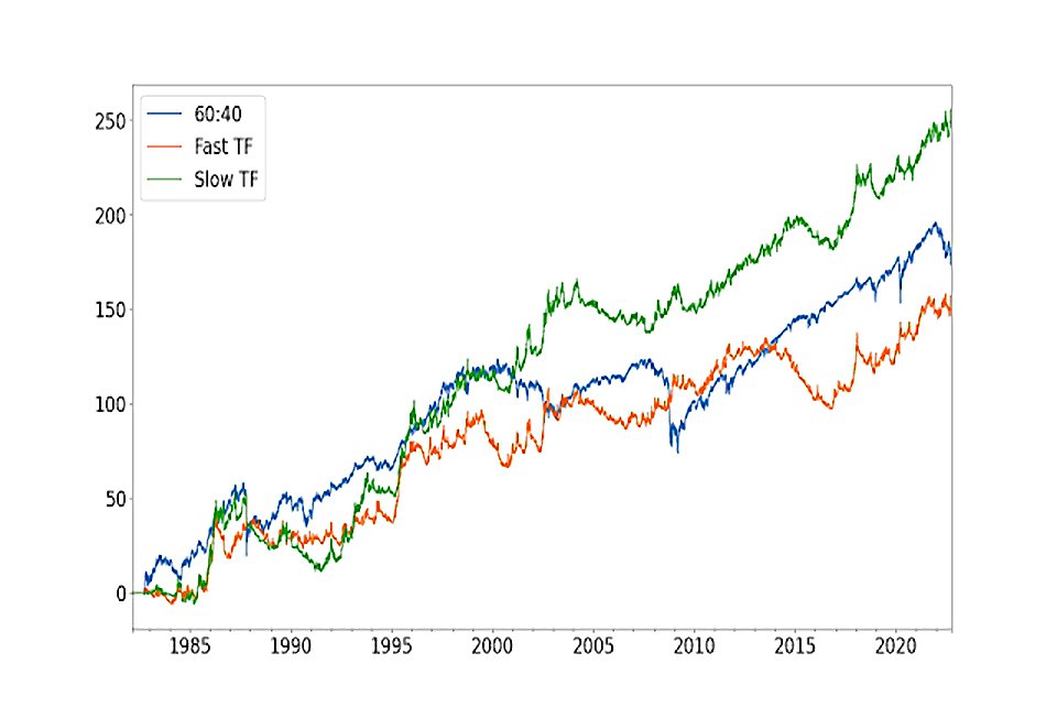
Rob looks at three assets:

1. A 60:40 long only portfolio of bonds and equities, represented by the US 10 year and S&P 500
2. A slow/medium speed trend following strategy, trading the US 10 year and S&P 500 future with equal risk allocation, with a 12% equity-like annualised risk target. This is a combination of EWMAC crossovers: 32,128 and 64,256
3. A relatively fast trend following strategy, trading the US 10 year and S&P 500 future with equal risk allocation, with a 12% annualised risk target. Again this is a combination of EWMAC crossovers: 8, 32 and 16,64

The trend assets are standardised at 12% annual vol to match the 60/40.

The long only strategy has nastier skew and worst tails than the fast trading
strategy, whilst the slow strategy comes somewhere in between.

Leaving out commodities from the trend assets means that the impact of real-world trend would be lower than in this analysis (which means a higher allocation to trend would be supported).

Demeaning

To compensate for the benign conditions during the period under analysis, Rob demeans the data.

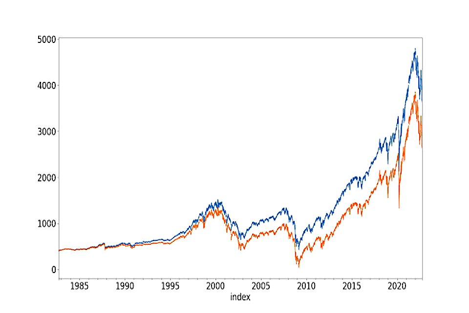
The P/E ratio in September 1982 was around 9.0, versus 20.1 now. This equates to 2.0% a year in returns coming from the rerating of equities. Over the same period US 10 year bond yields have fallen from around 10.2% to 4.0% now, equating to around 1.2% a year in returns.

The chart above shows the results for the S&P 500, and that below is for the US 10-year bond.

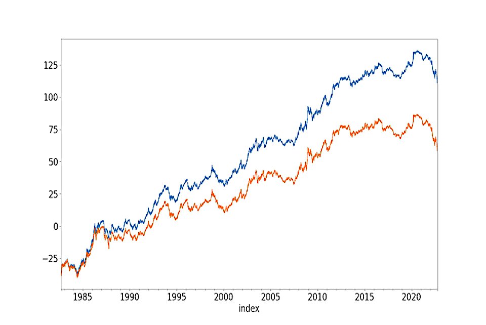
It doesn’t affect significantly standard deviations, skew, or tail ratios. But it does affect the Sharpe Ratio.

The SRs are lower.

The demeaning has a larger effect on the long only 60:40, and to a lesser extent the slower trend following. Both types of trend have become slightly less correlated with 60:40, which makes sense.

What to optimise?

Rob’s normal process would be to optimise for the SR and assume we can leverage as required but for this analysis, targeting returns with no leverage (CAGR) seems better.

That is effectively the same as maximising the (log) final value of your portfolio (Kelly criteria). Using geometric mean also means that negative skew and high kurtosis strategies will be punished, as will excessive standard deviation.

By assuming a CAGR maximiser, I don’t need to worry about the efficient frontier, I can maximise for a single point. It’s for this reason that I’ve created TF strategies with similar vol to 60:40.

To deal with uncertainty, Rob uses re-sampling:

I randomly sample from the joint distribution of daily returns for the three assets to create a new set of account curves. For a given set of instrument weights, I then measure the utility statistic (CAGR). I end up with a distribution of CAGR for a given set of weights.

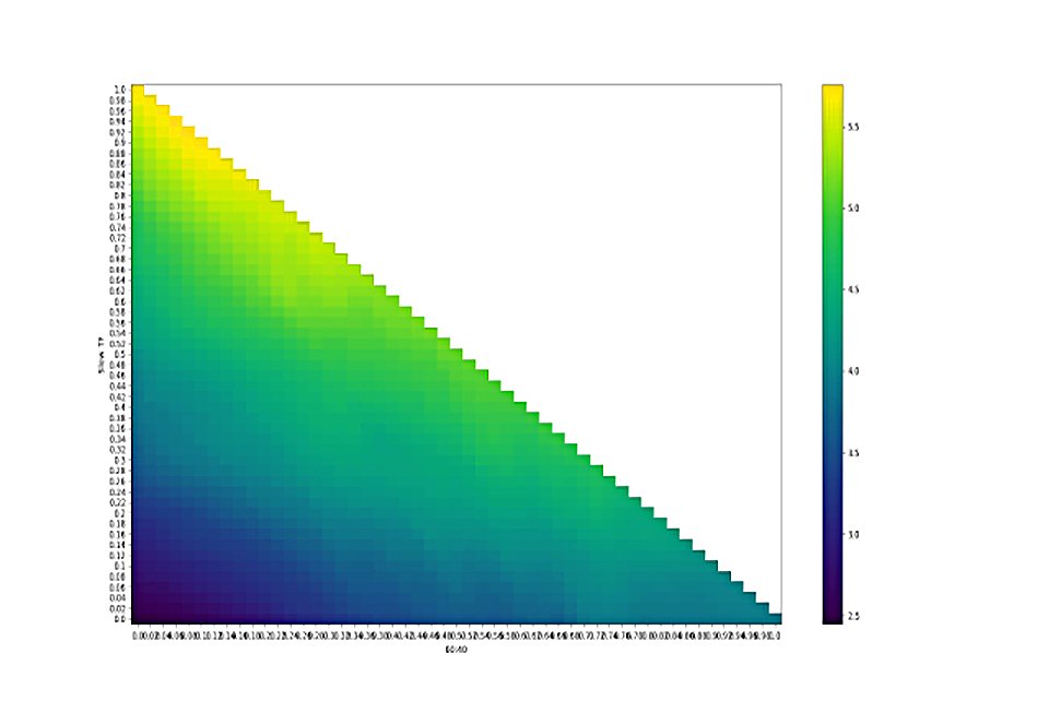
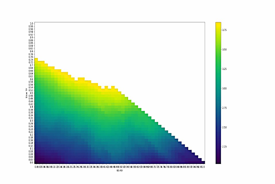
The colour shown reflects the CAGR. The x-axis is the weight for the long only 60:40 portfolio, and the y-axis for slow trend following. The weight to fast trend following will be whatever is left over.

The diagonal line from top left to bottom right is where there is zero weight to fast trend following; top left is 100% slow TF and bottom right is 100% long only.

The brightest yellow is at 94% slow TF and 6% long only, which is pretty extreme, but there’s a reasonably large range of yellow.

---

Rob calculates the 30% estimate for the optimal weight to have a CAGR of 4.36 and declares himself to be indifferent to any portfolio whose median CAGR is above this.

• Replacing these portfolios with white gives the following:

A weight of 30% in long only, 34% in slow trend following, and 36% in fast trend following; is just inside the whitespace. The maximum weight we can have to long only and still remain within this region (at the bottom right) is about 80%.

So the minimum trend allocation is 20%.

• Rob estimates the optimum as the centre of the whitespace below the diagonal, which is around 40% long, 50% slow TF and 10% fast TF.

That’s a lot of trend.

Without the following wind

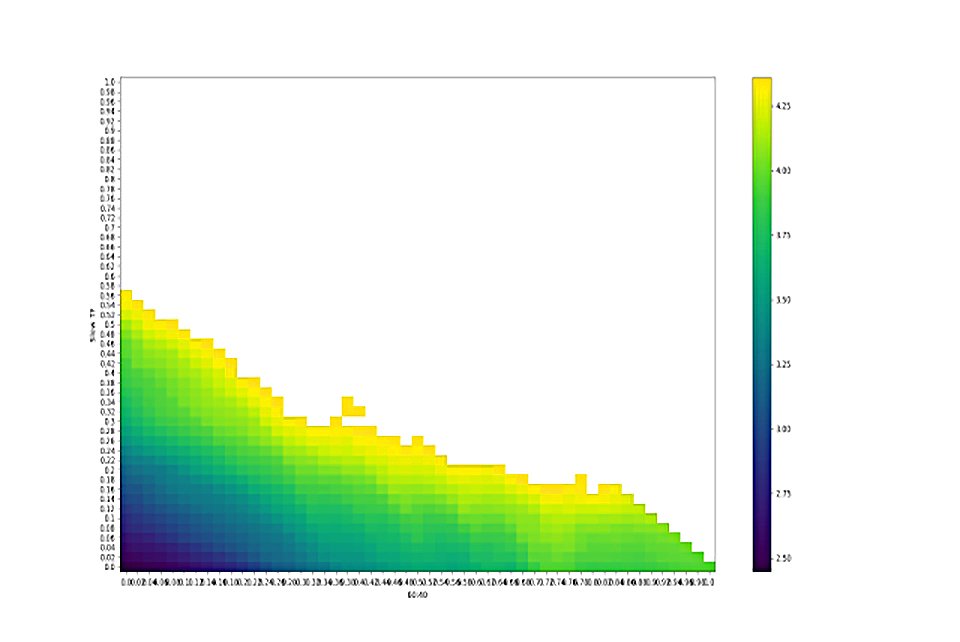
Here’s the same analysis on the demeaned data.

• The top left is now a lot better than the bottom right, implying a lower weight to 60/40.

In fact the optimal is 100% in slow trend following; zilch, nil, zero, nada in both fast TF and 60:40.

The whitespace area is much smaller this time and confined to the top right.

• Rob picks 45% long and 55% slow TF as a suitable portfolio.

The most you can have in 60:40 is now 45% (and so the minimum in trend is now 55%).

• The centre of the whitespace is around 20% long, 75% slow TF and 5% fast TF.

Conclusions

It’s great that Rob has worked through this analysis for us, but the resulting allocations are hard to implement.

• Not many more people will fancy 55% TF than will follow Jerry Parker into 100% TF.

Rob notes that his results depend on the finding that Slow TF has a higher SR than long only.

• Correcting for this would allocate more to both long and Fast TF.

The analysis could also be made a lot more realistic/complicated:

1. Add international stocks
2. Add bonds of different durations, plus corporates and linkers
3. Add other long-only portfolios (eg. risk parity variations)
4. Add more instruments (and fees) to the TF options

But Rob thinks that these changes would only increase the TF allocation.

---

So the real takeaway is that you should have as much trend as you can stomach, and/or practically implement.

• However far you get, the maths will be there to support you.

Ignoring tax considerations, I would like to be somewhere in the 10% to 33% range for trend (as I believe Rob himself is at present).

• But given the retail investing rules in the UK, that’s just a pipedream.

Until next time.