RP: Silver Bullet or Bridge Too Far?

Today’s post looks at a 2018 study from the CFA on Risk Parity.

Managing Muti-Asset Strategies

The study forms Chapter Four of a CFA publication called Managing Multi-Asset Strategies.

• It’s written by Gregory C Allen, whom I haven’t come across before.

I think this chapter was a reference in a Risk Parity Radio podcast episode from 2021, but I’m afraid I didn’t make a note of where I found it.

• The Chapter is called “Risk Parity: Silver Bullet or Bridge Too Far?”, and it looks at RP from a theoretical framework using modern portfolio theory (MPT).

The Risk Parity Portfolio

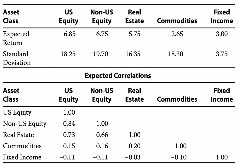
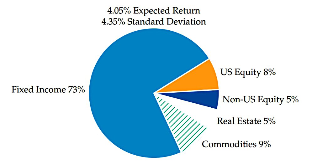
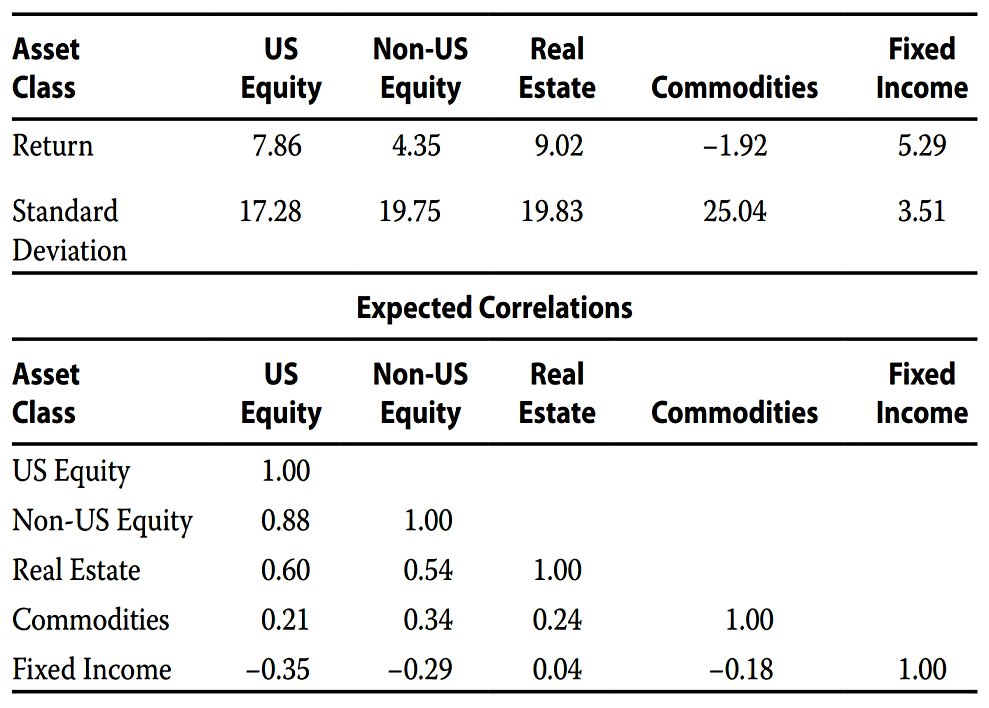
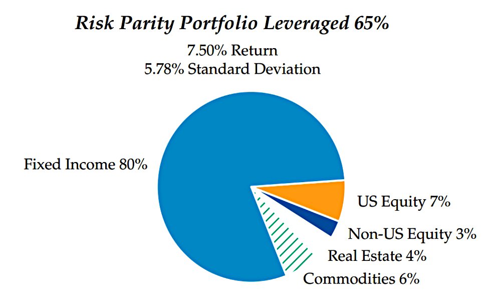
Using the returns, standard deviations and correlations above, Allen derives the Risk Parity (RP) portfolio shown below:

There is little consensus among practitioners on the exact methodology for determining the risk parity portfolio. I use standard deviation and correlation estimates to determine the marginal contribution of each asset class to overall portfolio risk [and] solve for the unique portfolio in which the marginal contributions of each asset class to total portfolio risk are equal.

Despite this, the fixed income allocation is higher than I would expect, at 73%.

Note that returns are only used to decide on the level of leverage – they do not affect allocations between assets.

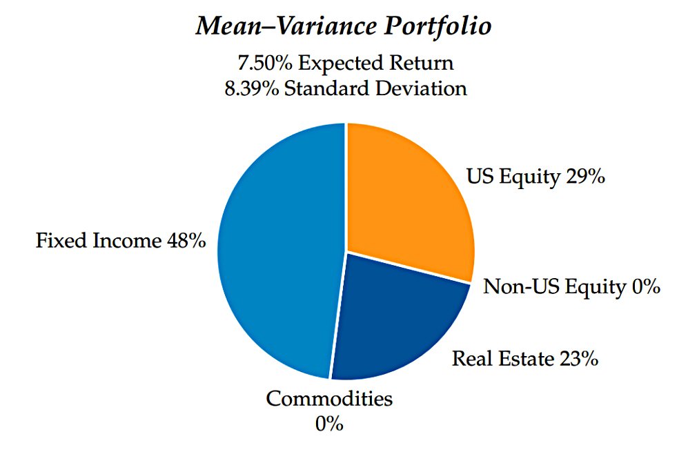
Mean-variance portfolio

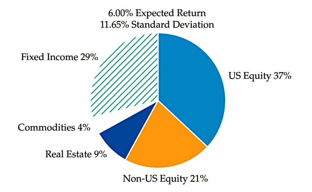
Allen provides a mean-variance portfolio (MVP) for comparison.

• This targets a 6% expected return and ends up close to a 70/30 stock/bond portfolio.
• The unlevered RP portfolio has an expected return that is 2% lower than this.

Allen says that the risk profile of the MVP is similar to that of the typical multi-asset portfolio used by institutional investors.

• Less than 5% of the volatility of this portfolio comes from fixed income.

Efficient frontier

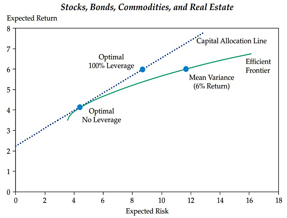
This chart shows the efficient frontier (green curve) which maps the expected (maximum) return from each level of risk (volatility).

• The MVP is plotted at the 6% return, 12% volatility point.

The straight line is the capital allocation line (CAL), which adds leverage to the classical modern portfolio theory (MPT).

• Leverage was added by Tobin in 1958.

The line intercepts the vertical axis at the borrowing rate (which is assumed to be 2.25% pa in this case).

• The slope of the line arises from finding the tangent to the efficient frontier.

This tangency point is the optimum portfolio (asset allocation) without leverage.

• We can move left on the CAL by adding cash to the optimum portfolio, and right up the CAL by adding leverage.

In this example, we need 100% leverage to raise the return of the optimal portfolio from 4% to the 6% available from the MVP.

• Note that this leveraged optimal portfolio (what I would call the RP portfolio) has a lower standard deviation (risk) – around 25% lower at 8.7% vs 11.7%.

Sub-optimal portfolios

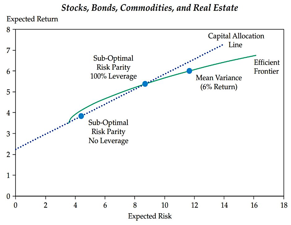
In the next section, Allen discusses sub-optimal portfolios – portfolios below the efficient frontier.

• He calls these RP portfolios, but for me, if we ignore the drag from implementation (costs, slippage etc), I would expect the unlevered RP portfolio to be close to the line.

In this example, 100% leverage only takes the sub-optimal portfolio back up to the efficient frontier, and an extra 30% of leverage would be needed to match the 6% pa return from the MVP.

• This extra leverage means that the levered sub-optimal portfolio is much closer in risk to the MVP (at the same level of return).

The takeaway is that in order to derive the full benefits of RP, we need to start out with an unlevered portfolio on the efficient frontier, or as Allen puts it:

Does it deliver the maximum expected return on an unlevered basis for its expected level of risk?

The second issue is the steepness of the CAL:

Is the borrowing rate sufficiently low relative to the premium for risky assets to warrant the use of leverage?

RP efficiency

Allen thinks that it is unlikely that the RP is on the efficient frontier because returns are not used to calculate it.

• I think this makes it unlikely that the RP and the MVP will be at the same point on the frontier, but doesn’t guarantee that the RP will be far from the frontier.

In practice, therefore, the question becomes, Is the risk parity portfolio a close enough approximation of the optimal portfolio to deliver on the promise of higher risk-adjusted returns?

Asness, Frazzini, and Pedersen (2012) have argued that the two portfolios are sufficiently similar.

This is a paper I will be looking at more closely in a subsequent post, but Allen summarises their argument as:

This is primarily because both portfolios overweight low-returning asset classes,  rather than there being something special about all asset classes contributing equal risk. The advantage of overweighting lower-returning asset classes is driven by a market inefficiency they call “leverage aversion”.

This means that some investors (including most PIs) overweight risky assets because they are averse to leverage (or cannot access it efficiently).

• This pushes up the prices of risky assets and gives them lower risk-adjusted returns.

Leverage

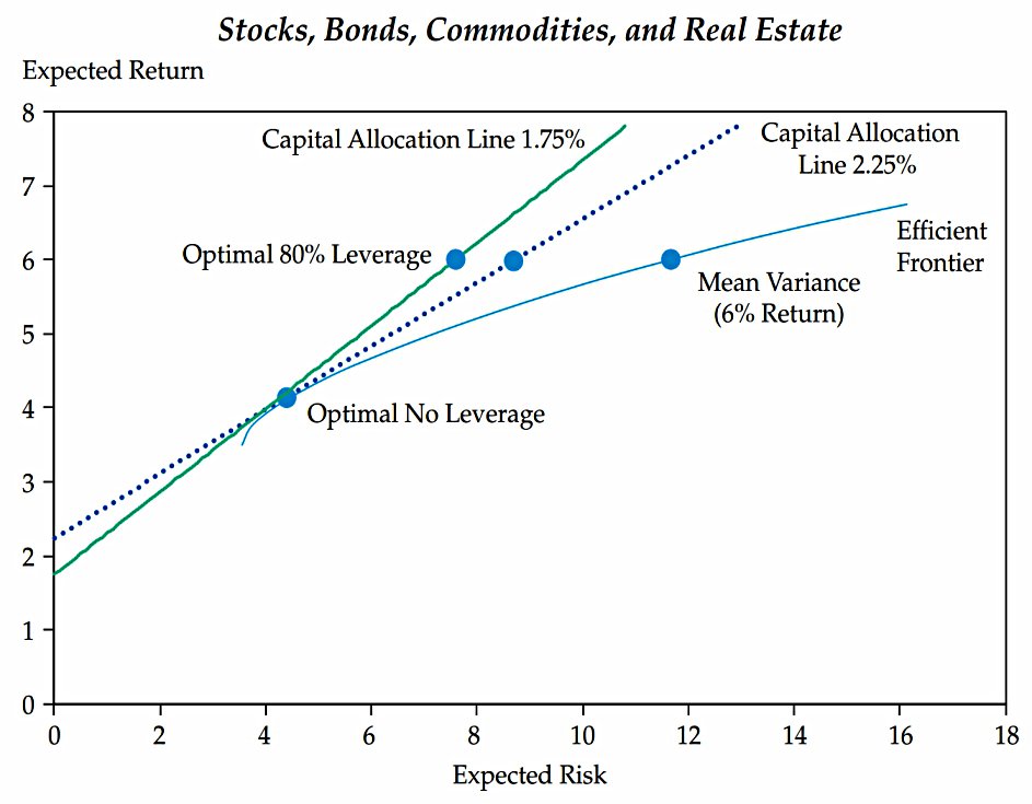
Allen notes that back in 1958, when Tobin added leverage to MPT, actually getting hold of it at a cost-effective rate was very difficult.

• But things have changed.

The cheaper the leverage, the better it works.

• The chart shows the difference between borrowing at 2.25% and at 1.75% pa.

The lower rate means that only 80% leverage is needed to match the MVP returns, and the risk reduction is increased.

---

But there have been changes on the asset side, too:

Quantitative easing and other macro factors [have] driven the expected premium for risky assets to very low levels. Furthermore, low yields combined with a historically high representation of government-backed bonds [have] driven the expected volatility of the bond market down to historical lows.

In RP, lower bond volatility means more bonds (so that they can equally contribute to risk).

• More bonds plus low returns from risk assets means low expected returns from RP, which means a flatter CAL and more leverage.

And the CAL line may curve (flatten) as the level of borrowing increases (as counterparties demand more compensation for increased credit risk). (( A negative yield curve can lead to a CAL that slopes down, as borrowing costs exceed long-term bond returns ))

Performance

RP delivers better risk-adjusted returns than the (unlevered) MVP – see eg. Asness et all (2012).

They simulated the performance of a risk parity portfolio relative to a 60/40 portfolio over 1926–2010 in the US market. They also analyzed 10 other developed markets globally over 1986–2010. In every case, the risk parity approach delivered higher risk-adjusted returns.

Allen provides data (in the table above) for 20 years to 2016.

Note that this was a particularly good time for risk parity, because the period was characterized by two major crises in the global equity markets: a consistently  upwardly sloping yield curve and a general decline in interest rates.

Neither portfolio closely resembles the portfolios used by large institutional investors over the last 20 years. The mean–variance portfolio benefits from knowing in advance the return patterns of each asset class and wisely assigns zero weights to both commodities.

The risk parity portfolio includes everything it is offered regardless of return but perfectly balances the marginal contribution to risk across the asset classes over the 20-year period. 

RP returns the same as MVP at 60% of the volatility, with a higher Sharpe (0.9 vs 0.6) and lower drawdowns.

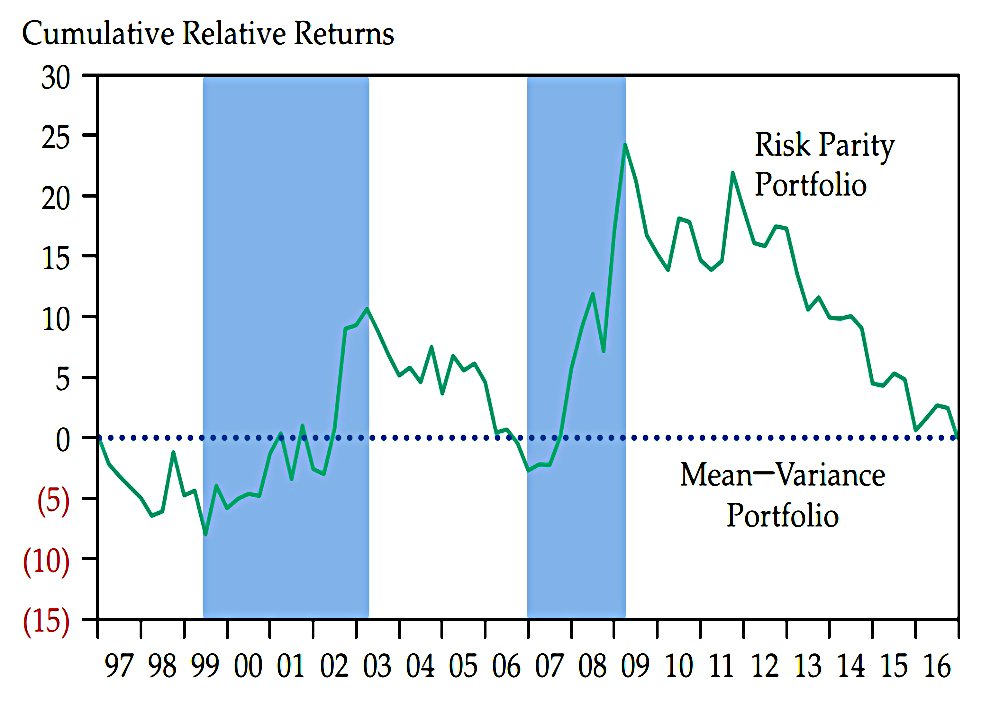
In this chart, the shaded areas are when RP outperforms MVP – the bad times for stocks.

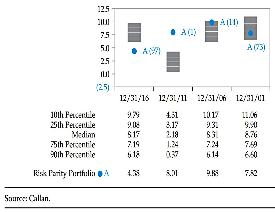
Allen compares the RP performance to institutional results from:

The Callan Total Fund Sponsor Database, a broad universe of over 1,500 public  and corporate pension funds, foundations, endowments, and other pools of institutional capital.

An RP portfolio would bounce around from the bottom to the top of the rankings.

• This makes RP attractive as a diversified to an MVP, rather than a direct alternative.

Allen notes that there has been almost no institutional adoption of RP as a sole strategy.

---

That’s it for today.

• RP clearly worked well – particularly as a diversifying strategy – when interest rates were falling and the yield curve sloped upwards.

As we potentially move into a period of rising interest rates and potential yield curve inversion, there will be questions asked about future performance.

• But interest rate risk is just one of many that RP is designed to cope with, and its supporters will argue that it will still deliver better risk-adjusted returns over the long run.

I’m half-convinced – enough to use RP as a diversifying strategy (amongst several) but not enough to commit fully.

• Until next time.