Tactical Asset Allocation – Meb Faber

Today’s post looks at a 2006 paper from Meb Faber on the subject of Tactical Asset Allocation.
Contents
Tactical Asset Allocation

We’ve met Meb several times before. (( In his writings only – not in real life ))
He’s also written a number of books and he has a podcast.
Today we’re looking at a very old paper of his called ” A Quantitative Approach to Tactical Asset Allocation”.
- My intro was slightly misleading in that the original paper was published in 2006 but Meb updated it in 2009 and 2013.
We’ll be looking at the 2013 version, which runs to 70 pages. The purpose of the paper is:
To present a simple quantitative method that improves the risk-adjusted returns across various asset classes.
The 2013 paper updates the original with data from 2008-12 and looks at how the method has worked out:
The models have performed well in real-time, achieving equity like returns with bond like volatility and drawdowns.
The paper also looks at elaborations of the original model, adding more asset classes and alternative weightings.
Risky Assets
In between versions of the paper, the 2008 crash happened.
- Meb observes that whilst risk assets (primarily stocks) will make you rich in the long term, they suffer from regular large drawdowns.
At such times, traditional diversification doesn’t help as much as it should, since correlations increase.
All of the G-7 countries have experienced at least one period where stocks lost 75% of their value. The unfortunate mathematics of a 75% decline require an investor to realize a 300% gain just to get back to even – the equivalent of compounding at 10% for 15 years!
CAPE
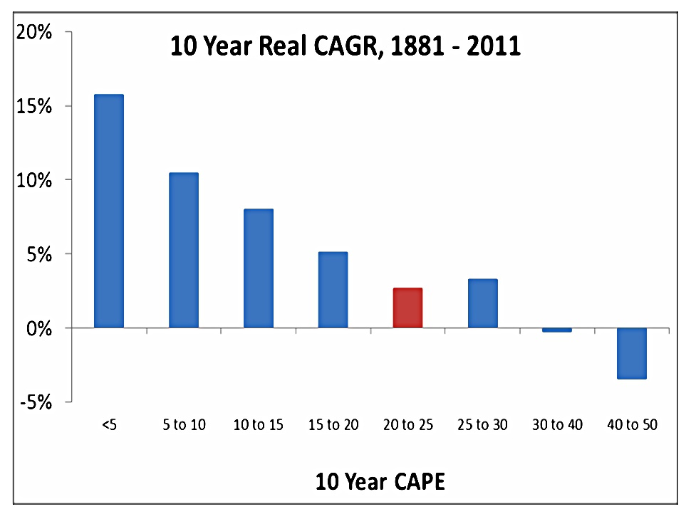
Meb also points out how high the CAPE was by 2012 (21.6, some 30% above the long-term average of 16.5).
- It’s got a lot higher since.
This matters because as CAPE rises, future 10-year returns decline.
- Today’s readings suggest slightly negative returns from stocks.
And bond returns are basically their yield, which for the US 10-year is 1.3% today (nominal – that’s a negative real yield).
- So a 60/40 portfolio might be expected to return around -2% pa real.
Back in 2013, Meb was predicting 1.4% real.
- It hasn’t quite worked out like that, but the subsequent outperformance only suggests that we’ve borrowed even more returns from our future.
Meb’s solution has two parts:
- We examine the effects of expanding a traditional 60/40 allocation into a more global allocation.
- We then overlay some simple risk management in hopes of protecting a portfolio against brutal bear markets.
Go Global
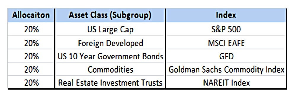
Meb’s original paper looked at five assets:
- US Large Cap, S&P 500
- Foreign Developed, MSCI EAFE
- US 10-Year Government Bonds
- Commodities, Goldman Sachs Commodity Index
- Real Estate Investment Trusts, NAREIT Index
Here are their returns from 1973 to 2012:
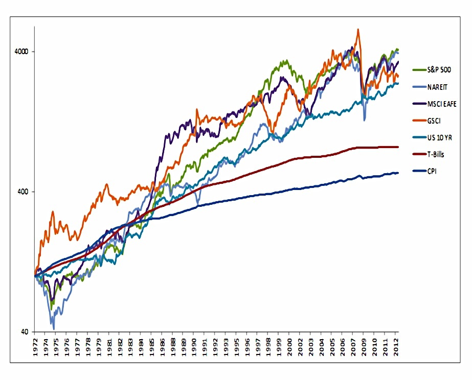
Most of the asset classes finished with similar returns over the time period. The exception was bonds, which trailed the other asset classes, an outcome that is to be expected due to their lower volatility and risk.
The fact that bonds were even close in absolute performance to the other equity-like asset classes reflects the greater than twenty year bull market that took yields from double-digit levels to near 2% today.
That 20+ year bull market in bonds is now close to 40 years old.
With the exception of U.S. government bonds, which declined less than 20%, the other four asset classes had drawdowns around 50% to 70%.
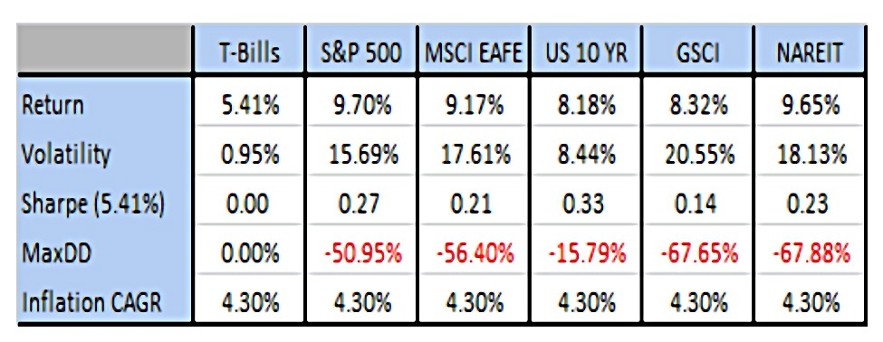
Meb also looked at Sharpe ratios:
Risky asset classes have Sharpe ratios that cluster around 0.20, while a diversified portfolio is around 0.40.
Manage your risk
This paper examines a very simple quantitative market-timing model that manages risk. A market timing solution is a risk-reduction technique that signals when an investor should exit a risky asset class in favor of risk-free investments.
Meb’s system is pretty simple, with a pair of rules applied to all asset classes:
- Buy when the price is above the 10-month (200-day) MA
- Sell and move to cash when the price is below the 200-day MA
The simple moving average is used, and the price check is only made on the last day of each month (at the close).
- The data series are total returns (including dividends).
- Cash returns are taken from 90-day T-bills.
S&P Timing
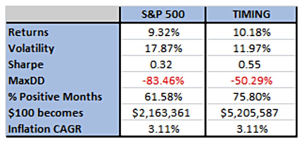
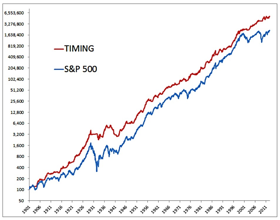
The first test of the system is the S&P 500 from 1901 to 2012:
The timing solution improved compounded returns while reducing risk [whilst] being invested in the market approximately 70% of the time and making less than one round-trip trade per year.
The Sharpe increases from 0.32 to 0.55.
Interestingly, the timing system underperforms in roughly 50% of years, but its lower volatility leads to higher compound returns.
The average return for the S&P 500 since 1901 was 11.26%, while timing the S&P 500 returned 11.22%. However, the compounded returns for the two are 9.32% and 10.18%, respectively.
Here the average is the arithmetic mean and the compound return is the geometric mean.
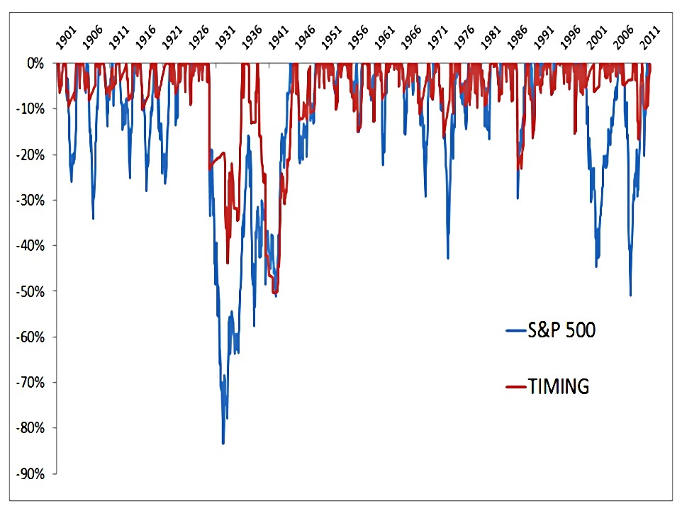
The 1930s bear market drawdown was reduced from 83.7% to 42.2%.
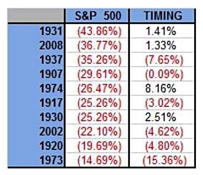
The table above shows the returns for the worst ten years for the S&P 500.
The correlation between negative years for the S&P 500 and the timing model is approximately -0.38, while the correlation for positive years is approximately 0.83. This reflects the ability of the timing model to stay long in up markets while exiting the long position during down markets.
Meb also provides a chart of the distribution of yearly returns:
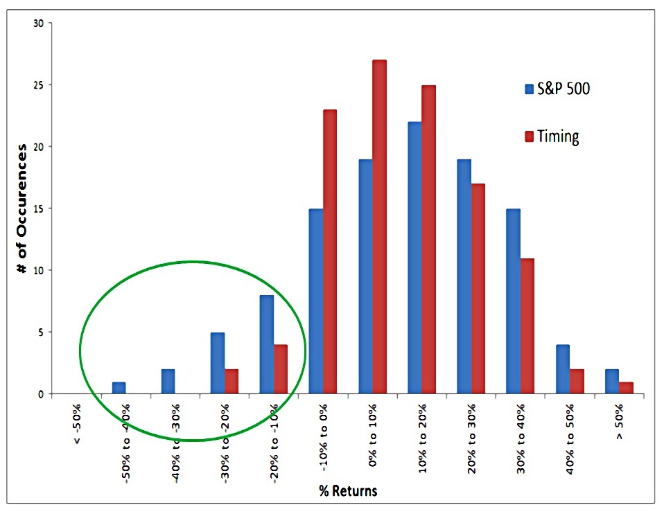
The timing system has fewer occurrences of both large gains and large losses, with correspondingly higher occurrences of small gains and losses. Most importantly, it avoids the far left tail of big negative losses.
The system also improves risk-adjusted returns in two-thirds of decades and improves drawdowns in all but two decades.
Global Tactical Asset Allocation
The next stage is to move to the five asset classes mentioned above, a model Meb refers to as GTAA.
The timing model uses equal weightings and treats each asset class independently – it is either long the asset class or in cash with its 20% allocation of the funds.
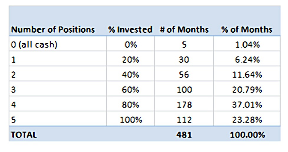
On average, the investor is 70% invested.
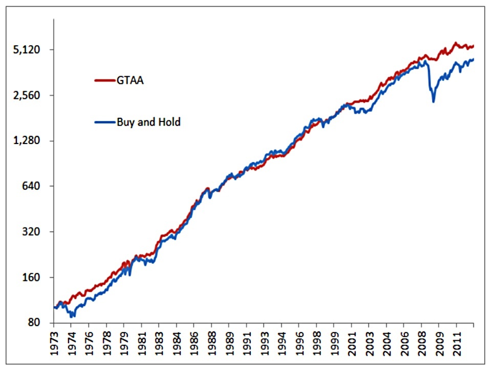
Equal-weighted five asset buy-and-hold does pretty well, but GTAA is better (by 2% pa).
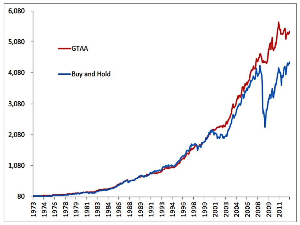
The outperformance is easier to see on a non-log scale.
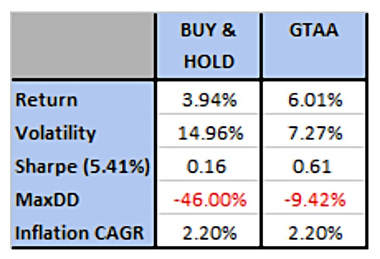
More importantly, volatility is down to 7.3% pa, the max drawdown is reduced by 80% (to 9.4%) and Sharpe is almost quadrupled (to 0.6).
- Note that the table above refers to the “out-of-sample” period from 2006 to 2012, but similar results are found over the entire period.
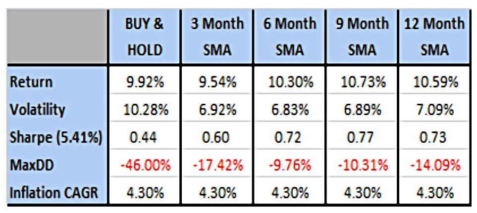
Meb also shows that any MA from 3 months to 12 months works well.
Practical considerations
Meb makes a couple of key points:
- Management fees should be identical for both the buy and hold and timing models
- Commissions should be a minimal factor due to the low turnover of the models.
- On average, the investor would be making three to four round-trip trades per year
Taxes could be an issue in the US, but probably not here in the UK.
- Even in the US, a tax-sheltered account could be used.
Volatility clustering
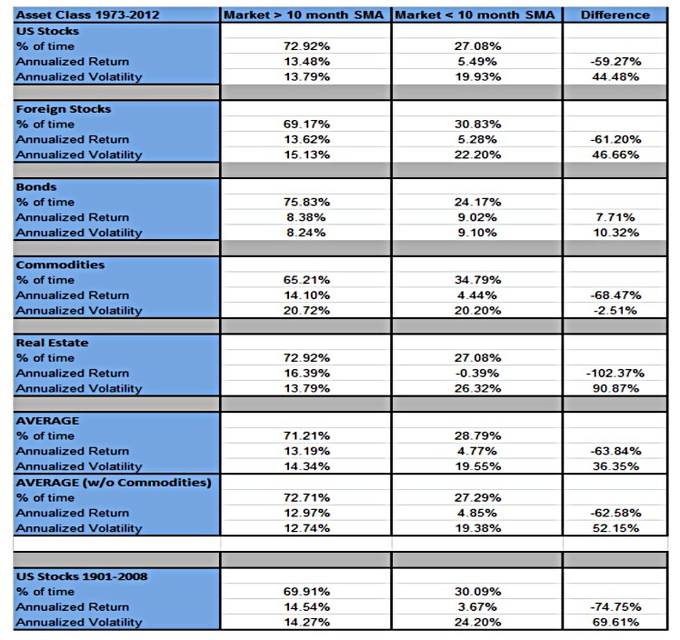
The system works because of volatility clustering:
On average, the returns are 60% lower and the volatility 30% higher when the market is below its 10-month simple moving average. Commodities are the one exception.
Variations
In the 2013 update to the paper, Meb provides some alternatives to the original GTAA approach.
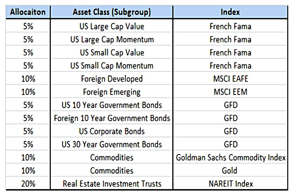
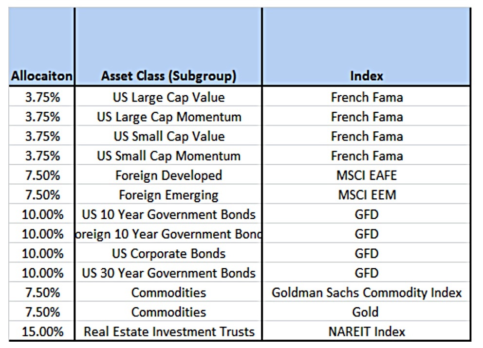
The first, despite his reservations, is a portfolio with more asset classes.
We believe there are only four real asset classes: stocks, bonds, commodities, and currencies. At the same time, expanding a portfolio with allocations less than 5% of the total does not do enough to move the needle on the entire portfolio’s risk and reward characteristics .
The thirteen-asset version of the strategy outperforms the five-asset version by 1.5% pa.
- Note that buy-and-hold with thirteen assets outperforms the 5-asset GTAA by 1% pa, and is only 0.5% pa behind the 13-asset GTAA.
Of course, GTAA-13 also show improvements in lower volatility, higher Sharpe and much lower max drawdowns.
The second variation was using 10-year Treasuries as the asset alternative instead of cash.
- This helped, even during periods of rising interest rates.
The third variation was a conservative GTAA with 40% in bonds.
- This compares well with the standard GTAA-13.
The fourth was an aggressive portfolio that selects the top 6 from the GTAA-13 ( ranked by an average of 1, 3, 6, and 12-month total returns/momentum).
- This is covered in detail in a paper we’ll cover in a future post, called “Relative Strength Strategies for Investing”.
The paper also looks at using just the top 3 assets, and at the use of leverage.
- All three of these approaches produce much higher returns (17.8% to 19.1% pa) at the expense of more volatility and higher max drawdowns.
Conclusions
It might be an old paper, but it’s a good one. As Meb says:
A non-discretionary, trendfollowing model acts as a risk-reduction technique with no adverse impact on return.
Diversification and the 200-day MA is all that you need to reduce volatility and max drawdowns.
- I look forward to the Relative Strength paper.
Until next time.
Mike Rawson
Mike is the owner of 7 Circles, and a private investor living in London. He has been managing his own money for 40 years, with some success.